Note
Access to this page requires authorization. You can try signing in or changing directories.
Access to this page requires authorization. You can try changing directories.
While the Fast Startup assessment is an easy way to get measurements in an easy to read report, it requires you to install the ADK, which takes some time to execute. It’s possible to quickly capture a Fast Startup trace using the Windows Performance Recorder (WPR) tool.
Step 1: Open Fast Startup trace using WPA
Open Windows Performance Recorder (WPR) from the Start menu
Modify the tracing configuration.
Select the First Level Triage and CPU Usage providers.
Change the performance scenario to Fast Startup.
Change the Number of iterations to 1 in order to gather a single trace.
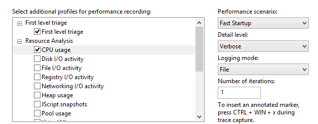
Click on Start.
Enter a path to save the resulting trace, and click on Save.
- This will force the system to reboot to gather and save the trace.
Once the system reboots, wait 5 minutes for tracing to finish.
You now have a trace that can be analyzed with Windows Performance Analyzer (WPA).
Step 2: Open Fast Startup trace using WPA
Open Windows Performance Analyzer (WPA) from the Start menu.
From the File menu, open the trace that you created in Step 1.
Open the Profiles menu, and click on Apply…
Click on Browse Catalog…
Select FastStartup.wpaprofile.
Click on Open.
You now have applied a visualization profile to the trace in order to get some commonly used graphs (CPU, disk, etc.).
Step 3: Visualize the activity timeline
Look at the Regions of Interest graph in the Deep Analysis tab
This view provides a timeline overview of all the Fast Startup subphases mentioned in Exercise 1.
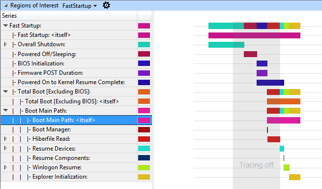
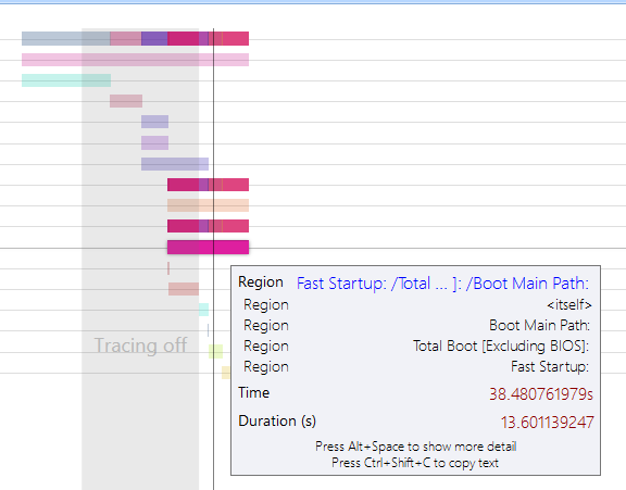
Hovering the mouse over a region bar causes a popup window to appear and provide more information for the region itself.
If you put the mouse over the Boot Main Path region, you can see its duration. In the example below, it lasts 13.6 seconds.
Take the time to navigate through the regions tree, and look at all the subphases to familiarize yourself with it.
The time that Explorer takes to initialize and finish is the time it takes to create the Windows desktop and make it visible to the user. This phase (and everything happening after, known as post on/off) can be impacted by processes started on boot.
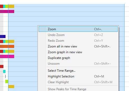
Select a 90 second interval starting at the beginning of Explorer Initialization and zoom in.
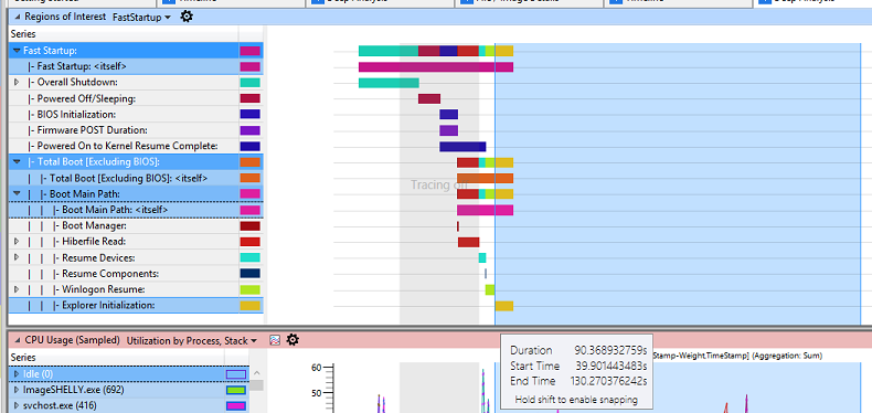
Under the Regions of Interest graph, there are two other valuable graphs: CPU Usage (sampled) and Disk usage. They will be used to evaluate the impact that the software preload has on post on/off resource consumption and responsiveness.
High CPU usage by applications and services can contribute to a poor user experience, such as UI unresponsiveness or video and sound glitches. When a single process uses too much CPU, other processes can be delayed because they must compete for system resources.
When a thread uses storage resources, it can increase the duration of the activity. When multiple threads contend for the use of storage, the resulting random disk seeks make delays more significant.
Step 4: Analyze process CPU usage
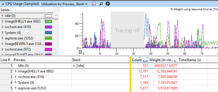
In order to evaluate how much CPU time is consumed by a process, focus on the CPU Usage (sampled) graph. The data that displays in the CPU Usage (Sampled) graph represents samples of CPU activity taken at regular 1 ms sampling intervals. Each row in the table represents a single sample.
Any CPU activity that occurs between samples is not recorded by this sampling method. Therefore, activities of very short duration such as interrupts are not well represented in the CPU Sampling graph.
Review the CPU usage for each process to identify the processes that have the highest CPU usage (Weight and %Weight). To do this, scroll down to the graph CPU Usage (sampled). On the left, view the list of processes. Each active process that is selected on the left displays on the graph.
**Tip: **
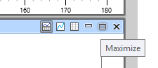
While using WPA graphs, you can change the view to display both the graph and the table. You can click the Maximize button to hide the other graphs displayed on the Analysis tab.
In this example, ImageSHELLY.exe consumes 12.4 seconds of CPU time over the interval of 90 seconds currently analyzed. Since the CPU on this system has two cores, this represents a relative percentage of utilization of 6.9%.
Using this information, you can investigate the specific process that is causing this CPU consumption, or forward these details to the developer who owns this process.
You can add additional columns to extract more information (right-click on the table column headers):
Thread ID: Identifier of the thread causing CPU usage
Stack: Call stack that highlights the code paths and functions that are causing CPU usage
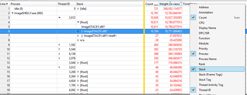
In the example above, there is only one thread causing most of the CPU usage within the ImageSHELLY.exe process: Thread 2612, with 10.77 seconds of CPU activity.
The stack shows that this activity is coming from the ImageSTACEY.dll module.
Step 5: Analyze process disk usage
In order to evaluate how much disk bandwidth is consumed by a process, focus on the Disk Usage graph.
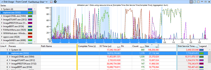
The columns of interest are:
Pri: Priority of the disk I/O. The three possible priority levels are: normal, low, and very low.
IO Type: Type of the I/O. The three possible I/O types are: read, write, and flush.
Process: Identifier of the process that created the disk I/O.
Path Tree: Structured tree that represents the locations of the files accessed by the I/O.
Size: Size (in bytes) of the I/O.
Disk Service time: Amount of time that it takes for the disk to service the I/O.
IO Time: Amount of time that the I/O spent in the Windows I/O queue.
- IO Time is always longer than Disk Service Time because an I/O can be queued when there is disk contention or when an I/O dispatcher at a higher priority must be completed first.
Add these columns and arrange them to obtain this view:
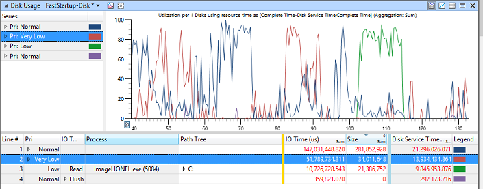
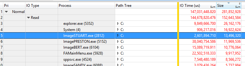
Post on/off only takes into account normal priority I/Os. Investigate the information about those disk reads according to process. Disk reads usually account for more disk access time than disk writes on boot, as a lot of data must be read from disk in order to launch processes and services.
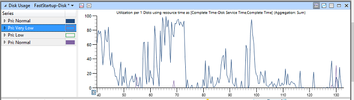
Click the color markers beside the Pri: Very Low and Pri: Low series so that only the normal priority I/Os are visible on the graph.
In the table view, expand the Normal priority row.
In the table view, expand the rows for Write, Read, and Flush, and then click the header for the Size column to sort the contents in decreasing order.
Your screen should look something like this:
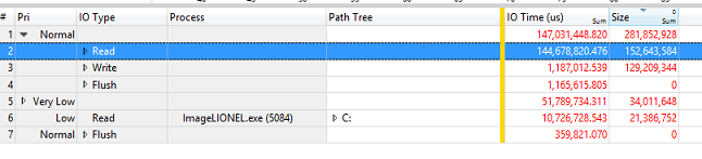
The preceding example shows the following:
152 MB of data was read from disk at normal priority.
129 MB of data was written to disk at normal priority.
- Those are mainly disk writes to persist the captured ETL trace file on storage.
In the table view, expand the Read IO Type row.
- You should now be able to see the processes that caused the largest amount of read disk I/O during post on/off.
Identify the top three processes that are contributing to disk reads and that are not Windows components.
In the table view, expand the Path Tree row for ImageSTUART.exe, and navigate through it.
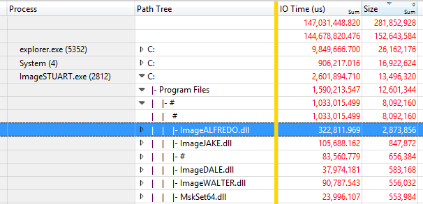
In the preceding example, ImageSTUART.exe reads 13.5 MB of data from disk when launched during post on/off, and most of the accesses are made reading DLL components in the Program Files folder.
Using this information, a software developer should identify his components and processes, and determine if the component size can be reduced, or if the launch code path can be optimized to minimize the amount of data read from disk.
You can also use this data to identify the 3rd party processes that launched on boot and is causing high disk usage. If a process appears to be introducing disk contention, it can then be removed from the image or simply not started at boot time.