Note
Access to this page requires authorization. You can try signing in or changing directories.
Access to this page requires authorization. You can try changing directories.
This article provides recommendations for capacity planning for Active Directory Domain Services (AD DS).
Goals of capacity planning
Capacity planning isn't the same as troubleshooting performance incidents. The goals of capacity planning are:
- Properly implement and operate an environment.
- Minimize time spent troubleshooting performance issues.
In capacity planning, an organization might have a baseline target of 40% processor utilization during peak periods to meet client performance requirements and give enough time to upgrade the hardware in the datacenter. Meanwhile, they set their monitoring alert threshold for performance issues at 90% over a five-minute interval.
When you continually exceed the capacity management threshold, then either adding more or faster processors to increase capacity or scaling the service across multiple servers would be a solution. Performance alert thresholds let you know when you need to take immediate action when performance issues negatively affect client experience. In contrast, a troubleshooting solution would be more concerned with addressing one-time events.
Capacity management is like the preventative measures you'd take to avoid a car accident, such as defensive driving, making sure the brakes are working properly, and so on. Performance troubleshooting is more like when the police, fire department, and emergency medical professionals respond to an accident.
Over the last several years, capacity planning guidance for scale-up systems has changed dramatically. The following changes in system architectures challenge fundamental assumptions about designing and scaling a service:
- 64-bit server platforms
- Virtualization
- Increased attention to power consumption
- SSD storage
- Cloud scenarios
The approach to capacity planning is also shifting from server-based planning exercises to service-based ones. Active Directory Domain Services (AD DS), a mature distributed service that many Microsoft and third-party products use as a backend, is now one the most critical products in ensuring your other applications have the necessary capacity to run.
Important information to consider before you start planning
In order to get the most out of this article, you should do the following things:
- Make sure you've read and understand the Performance Tuning Guidelines for Windows Server 2012 R2.
- Understand that the Windows Server platform is an x64-based architecture. Also, you must understand that this article's guidelines still apply even if your Active Directory environment is installed on Windows Server 2003 x86 (now beyond the end of the support lifecycle) and has a directory information tree (DIT) that's smaller than 1.5 GB and can easily be stored in memory.
- Understand that capacity planning is a continuous process, so you should regularly review how well the environment you build is meeting your expectations.
- Understand that optimization occurs over multiple hardware lifecycles as hardware costs change. For example, if memory becomes cheaper, cost per core decreases, or the price of different storage options change.
- Plan for the peak busy period of every day. We recommend you make your plans based on either 30 minute or hour intervals. Intervals greater than one hour may hide when your service actually reaches peak capacity, and intervals less than 30 minutes can give you inaccurate information that makes transient increases look more important than they actually are.
- Plan for growth over the course of the hardware lifecycle for the enterprise. This planning can include strategies for upgrading or adding hardware in a staggered fashion, or a complete refresh every three to five years. Each growth plan requires you estimate how much the load on Active Directory grows. Historical data can help you make a more accurate assessment.
- Plan for fault tolerance. Once you've derived the estimate N, plan for scenarios that include N - 1, N - 2, and N - x.
Based on your growth plan, add extra servers according to organizational need to ensure that losing one or more servers doesn't cause the system to exceed maximum peak capacity estimates.
Also remember that you must integrate your growth and fault tolerance plans. For example, if you know your deployment currently requires one domain controller (DC) to support the load but your estimate says the load will double in the next year and require two DCs to carry, then your system doesn't have enough capacity to support fault tolerance. In order to prevent this lack of capacity, you should instead plan to start with three DCs. If your budget doesn't allow for three DCs, you can also start with two DCs, then plan to add a third after three or six months.
Note
Adding Active Directory-aware applications might have a noticeable impact on the DC load, whether the load is coming from the application servers or clients.
The three-part capacity planning cycle
Before you start your planning cycle, you need to decide what quality of service your organization requires. All recommendations and guidance in this article are for optimal performance environments. However, you can selectively relax them in cases where you don't need optimization. For example, if your organization needs a higher level of concurrency and more consistent user experience, you should look at setting up a datacenter. Datacenters let you pay greater attention to redundancy and minimize system and infrastructure bottlenecks. In contrast, if you're planning a deployment for a satellite office with only a few users, you don't need to worry as much about hardware and infrastructure optimization, which lets you choose lower-cost options.
Next, you should decide whether to go with virtual or physical machines. From a capacity planning standpoint, there's no right or wrong answer. However, you do need to keep in mind that each scenario gives you a different set of variables to work with.
Virtualization scenarios give you two options:
- Direct mapping, where you have only one guest per host.
- Shared host scenarios, where you have multiple guests per host.
You can treat direct mapping scenarios identically to physical hosts. If you choose a shared host scenario, it introduces other variables that you should take into consideration in later sections. Shared hosts also compete for resources with Active Directory Domain Services (AD DS), which may affect system performance and user experience.
Now that we've answered those questions, let's look at the capacity planning cycle itself. Each capacity planning cycle involves a three-step process:
- Measure the existing environment, determine where the system bottlenecks currently are, and get environmental basics necessary to plan the amount of capacity your deployment needs.
- Determine what hardware you need based on your capacity requirements.
- Monitor and validate that the infrastructure you set up is operating within specifications. Data you collect in this step becomes the baseline for the next cycle of capacity planning.
Applying the process
To optimize performance, ensure the following major components are correctly selected and tuned to the application loads:
- Memory
- Network
- Storage
- Processor
- Netlogon
Basic storage requirements for AD DS and the general behavior of compatible client software allow environments with as many as 10,000 to 20,000 users to ignore capacity planning for physical hardware, as most modern server-class systems can already handle a load that size. However, the tables in Data collection summary tables explain how to evaluate your existing environment to select the right hardware. The sections after that one go into more detail about baseline recommendations and environment-specific principles for hardware to help AD DS admins evaluate their infrastructure.
Other information you should keep in mind while planning:
- Any sizing based on current data is only accurate for the current environment.
- When making estimates, expect demand to grow over the lifecycle of the hardware.
- Accommodate future growth by determining whether you should oversize your environment today or gradually add capacity over the course of the lifecycle.
- All capacity planning principles and methodologies you'd apply to a physical deployment also apply to a virtualized deployment. However, when planning a virtualized environment, you need to remember to add the virtualization overhead to any domain-related planning or estimates.
- Capacity planning is a prediction, not a perfectly correct value, so don't expect it to be perfectly accurate. Always remember to adjust capacity as needed and constantly validate that your environment is working as intended.
Data collection summary tables
The following tables list and explain criteria for determining your hardware estimates.
Working environment
| Component | Estimates |
|---|---|
| Storage/Database Size | 40 KB to 60 KB for each user |
| RAM | Database Size Base operating system recommendations Third-party applications |
| Network | 1 GB |
| CPU | 1,000 concurrent users for each core |
High-level evaluation criteria
| Component | Evaluation criteria | Planning considerations |
|---|---|---|
| Storage/database size | Offline defragmentation | |
| Storage/database performance |
|
|
| RAM |
|
|
| Network |
|
|
| CPU |
|
|
| NetLogon |
|
|
Planning
For a long time, the usual recommendation for AD DS sizing was to put in as much RAM as the database size. Now that AD DS environments and the ecosystem that consumes them have grown much larger, things have changed. Although increased compute power and switching from x86 architecture to x64 made subtler aspects of sizing for performance irrelevant to customers running AD DS on physical machines, virtualization has made a tuning a much bigger concern.
To address those concerns, the following sections describe how to determine and plan for the demands of Active Directory as a service. You can apply these guidelines to any environment regardless of whether your environment is physical, virtualized, or mixed. To maximize your performance, your goal should be to get your AD DS environment as close to processor bound as possible.
RAM
The more storage you can cache in the RAM, the less needs to go to disk. To maximize server scalability, the minimum amount of RAM you use should equal the sum of the current database size, the total system value size, the recommended amount for your operating system, and the vendor recommendations for the agents (antivirus programs, monitoring, backup, and so on). You should also include extra RAM to accommodate future growth over the server's lifetime. This estimate will change based on database growth and environmental changes.
For environments where maximizing RAM is either not cost-effective or unfeasible, such as satellite locations or when the Directory Information Tree (DIT) is too large, skip ahead to Storage to make sure your storage is configured properly.
Another important thing to consider for sizing memory is the page file sizing. In disk sizing, like everything else related to memory, the goal is to minimize disk usage. In particular, how much RAM do you need to minimize paging? The next few sections should give you the information you need to answer this question. Other considerations for page size that don't necessarily affect AD DS performance are operating system (OS) recommendations and configuring your system for memory dumps.
Determining how much RAM a domain controller (DC) needs can be difficult due to many complex factors:
- Existing systems aren't always reliable indicators of RAM requirements because the Local Security Authority Subsystem Service (LSSAS) trims RAM under memory pressure conditions, artificially deflating requirements.
- Individual DCs only need to cache data their clients are interested in. This means data cached in different environments will change depending on what kinds of clients it contains. For example, a DC in an environment with an Exchange Server will collect different data than a DC that only authenticates users.
- The amount of effort you need to evaluate RAM for each DC on a case-by-case basis is often excessive and changes as the environment changes.
The criteria behind recommendations can help you make more informed decisions:
- The more you cache in RAM, the less you need to go to disk.
- Storage is a computer's slowest component. Data access on spindle-based and SSD storage media is a million times slower than data access in RAM.
Virtualization considerations for RAM
Your goal for optimizing RAM is to minimize the amount of time spent going to disk. You should also avoid memory over-commit at the host. In virtualization scenarios, memory over-commit is when the system allocates more RAM to guests than what exists on the physical machine itself. While over-commit isn't a problem on its own, when the total memory used by all guests exceeds the capability of the host's RAM, it causes the host to page. Paging makes performance disk-bound in cases where the DC goes to the NTDS.nit or page file to get data or the host goes to disk to try to access RAM data. As a result, this process vastly decreases performance and overall user experience.
Calculation summary example
| Component | Estimated memory (example) |
|---|---|
| Base operating system recommended RAM (Windows Server 2008) | 2 GB |
| LSASS internal tasks | 200 MB |
| Monitoring agent | 100 MB |
| Antivirus | 100 MB |
| Database (Global Catalog) | 8.5 GB |
| Cushion for backup to run, administrators to log on without impact | 1 GB |
| Total | 12 GB |
Recommended: 16 GB
Over time, more data is added to the database, and the average server lifespan is about three to five years. Based on a growth estimate of 333%, 16 GB is a reasonable amount of RAM to put in a physical server.
Network
This section is about evaluating how much total bandwidth and network capacity your deployment needs, inclusive of client queries, Group Policy settings, and so on. You can collect data to make your estimate by using the Network Interface(*)\Bytes Received/sec and Network Interface(*)\Bytes Sent/sec performance counters. Sample intervals for Network Interface counters should be either 15, 30, or 60 minutes. Anything less will be too volatile for good measurements, and anything greater will excessively smooth out daily peaks.
Note
Generally, the majority of network traffic on a DC is outbound as the DC responds to client queries. As a result, this section mainly focuses on outbound traffic. However, we also recommend you also evaluate each of your environments for inbound traffic. You can use the guidelines in this article to evaluate inbound network traffic requirements as well. For more information, see 929851: The default dynamic port range for TCP/IP has changed in Windows Vista and in Windows Server 2008.
Bandwidth needs
Planning for network scalability covers two distinct categories: the amount of traffic and the CPU load from the network traffic.
There are two things you need to take into account when capacity planning for traffic support. First, you need to know how much Active Directory Replication Traffic goes between your DCs. Second, you must evaluate your intrasite client-to-server traffic. Intrasite traffic mainly receives small requests from clients relative to the large amounts of data it sends back to clients. 100 MB is usually enough for environments with up to 5,000 users per server. For environments of over 5,000 users, we recommend you use a 1 GB network adapter and Receive Side Scaling (RSS) support instead.
To evaluate intrasite traffic capacity, particularly in server consolidation scenarios, you should look at the Network Interface(*)\Bytes/sec performance counter across all DCs in a site, add them together, then divide the sum by the target number of DCs. An easy way to calculate this number is to open the Windows Reliability and Performance Monitor and look at the Stacked Area view. Make sure all the counters are scaled the same.
Let's take a look at an example of a more complex way to validate that this general rule applies to a specific environment. In this example, we're making the following assumptions:
- The goal is to reduce the footprint to as few servers as possible. Ideally, one server carries the load, then you deploy an additional server for redundancy (n + 1 scenario).
- In this scenario, the current network adapter only supports 100 MB and is in a switched environment.
- The maximum target network bandwidth utilization is 60% in an n scenario (loss of a DC).
- Each server has about 10,000 clients connected to it.
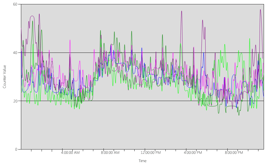
Now, let's take a look at what the chart in the Network Interface(*)\Bytes Sent/sec counter says about this example scenario:
- The business day starts ramping up around 5:30 AM and winds down at 7:00 PM.
- The peak busiest period is from 8:00 AM to 8:15 AM, with greater than 25 bytes sent per second on the busiest DC.
Note
All performance data is historical, so the peak data point at 8:15 AM indicates the load from 8:00 AM to 8:15 AM.
- There are spikes before 4:00 AM, with more than 20 bytes sent per second on the busiest DC, which could indicate either load from different time zones or background infrastructure activity, such as backups. Since the peak at 8:00 AM exceeds this activity, it's not relevant.
- There are five DCs in the site.
- The maximum load is about 5.5 MBps per DC, which represents 44% of the 100 MB connection. Using this data, we can estimate that the total bandwidth needed between 8:00 AM and 8:15 AM is 28 MBps.
Note
The Network Interface send/receive counters are in bytes, but the network bandwidth is measured in bits. Therefore, to calculate the total bandwidth, you'd need to do 100 MB ÷ 8 = 12.5 MB and 1 GB ÷ 8 = 128 MB.
Now that we've reviewed the data, what conclusions can we draw from it?
- The current environment meets the n + 1 level of fault tolerance at 60% target utilization. Taking one system offline will shift the bandwidth per server from about 5.5 MBps (44%) to about 7 MBps (56%).
- Based on the previously stated goal of consolidating to one server, this change exceeds the maximum target utilization and possible utilization of a 100 MB connection.
- With a 1 GB connection, this value represents 22% of the total capacity.
- Under normal operating conditions in the n + 1 scenario, the client load is relatively evenly distributed at about 14 MBps per server or 11% of total capacity.
- To make sure you have enough capacity while a DC is unavailable, the normal operating targets per server would be about 30% network utilization or 38 MBps per server. Failover targets would be 60% network utilization or 72 MBps per server.
The final system deployment must have 1 GB network adapter and a connection to a network infrastructure that will support said load. Because of the amount of network traffic, the CPU load from network communications can potentially limit the maximum scalability of AD DS. You can use this same process to estimate inbound communication to the DC. However, in most scenarios, you won't need to calculate the inbound traffic because it's smaller than the outbound traffic.
It's important to make sure your hardware supports RSS in environments with over 5,000 users per server. For high network traffic scenarios, balancing interrupt load can be a bottleneck. You can detect potential bottlenecks by checking the Processor(*)\% Interrupt Time counter to see if interrupt time is unevenly distributed across CPUs. RSS-enabled network interface controllers (NICs) can mitigate these limitations and increase scalability.
Note
You can take a similar approach to estimate if you need more capacity when consolidating datacenters or retiring a DC in a satellite location. To estimate the required capacity, simply look at the data for outbound and inbound traffic to clients. The result is the amount od traffic present in the wide area network (WAN) links.
In some cases, you might experience more traffic than expected because traffic is slower, such as when certificate checking fails to meet aggressive time-outs on the WAN. For this reason, WAN sizing and utilization should be an iterative, ongoing process.
Virtualization considerations for network bandwidth
The typical recommendations for a physical server are 1 GB for servers supporting over 5,000 users. Once multiple guests start sharing an underlying virtual switch infrastructure, you should pay extra attention to whether the host has adequate network bandwidth to support all the guests in the system. You need to consider bandwidth regardless of whether the network includes the DC running as a VM on a host with network traffic going over a virtual switch or directly connected to a physical switch. Virtual switches are components where the uplink must support the amount of data the connection transmits, which means the physical host network adapter linked to the switch should be able to support the DC load plus all other guests sharing the virtual switch connected to the physical network adapter.
Network calculation summary example
The following table contains values from an example scenario that we can use to calculate network capacity:
| System | Peak bandwidth |
|---|---|
| DC 1 | 6.5 MBps |
| DC 2 | 6.25 MBps |
| DC 3 | 6.25 MBps |
| DC 4 | 5.75 MBps |
| DC 5 | 4.75 MBps |
| Total | 28.5 MBps |
Based on this table, the recommended bandwidth would be 72 MBps (28.5 MBps ÷ 40%).
| Target system count | Total bandwidth (from above) |
|---|---|
| 2 | 28.5 MBps |
| Resulting normal behavior | 28.5 ÷ 2 = 14.25 MBps |
As always, you should assume that client load will increase over time, so you should plan for this growth as early as possible. We recommend you plan for at least 50% estimated network traffic growth.
Storage
There are two things you should consider when capacity planning for storage:
- Capacity or storage size
- Performance
Although capacity is important, it's important to not neglect performance. With current hardware costs, most environments aren't large enough for either factor to be a major concern. Therefore, the usual recommendation is to just put in as much RAM as the database size. However, this recommendation might be overkill for satellite locations in larger environments.
Sizing
Evaluating for storage
Compared to when Active Directory first arrived at a time when 4 GB and 9 GB drives were the most common drive sizes, now sizing for Active Directory isn't even a consideration for all but the largest environments. With the smallest available hard drive sizes in the 180 GB range, the entire operating system, SYSVOL, and NTDS.dit can easily fit on one drive. As a result, we recommend you avoid investing too heavily in this area.
Our only recommendation is that you ensure 110% of the NTS.dit size is available so you can defragment your storage. Beyond that, you should take the usual considerations in accommodating future growth.
If you are going to evaluate your storage, then first you must evaluate how large the NTDS.dit and SYSVOL need to be. These measurements will help you size both the fixed disk and RAM allocations. Because the components are relatively low cost, you don't need to be super precise when doing the math. For more information about storage evaluation, see Storage Limits and Growth Estimates for Active Directory Users and Organizational Units.
Note
The articles linked in the previous paragraph are based on data size estimates made during the release of Active Directory in Windows 2000. When making your own estimate, use object sizes that reflect the actual size of objects in your environment.
As you review existing environments with multiple domains, you may notice variations in database sizes. When you spot these variations, use the smallest global catalog (GC) and non-GC sizes.
Database sizes can vary between OS versions. DCs running earlier OS versions like Windows Server 2003 have smaller database sizes than one running a later version like Windows Server 2008 R2. The DC having features like Active Directory REcycle Bin or Credential Roaming enabled can also affect database size.
Note
- For new environments, remember that 100,000 users in the same domain consume about 450 MB of space. The attributes you populate can have a huge impact on the total amount of space consumed. Attributes are populated by many objects from both third-party and Microsoft products, including Microsoft Exchange Server and Lync. As a result, we recommend you evaluate based on the environment's product portfolio. However, you should also keep in mind that doing the math and testing for precise estimates for all but the largest environments may not be worth significant time or effort.
- Make sure the free space you have available is 110% of the NTDS.dit size to enable offline defrag. This free space also lets you plan for growth over the server's three to five year hardware lifespan. If you have the storage for it, allocating enough free space to equal 300% of the DIT for storage is a safe way to accommodate growth and defragging.
Virtualization considerations for storage
In scenarios where you allocate multiple Virtual Hard Disk (VHD) files to a single volume, you should use a fixed state disk of at least 210% the size of the DIT (100% of the DIT + 110% free space) to ensure you have enough space reserved for your needs.
Storage calculation summary example
The following table lists the values you'd use to estimate the space requirements for a hypothetical storage scenario.
| Data collected from evaluation phase | Size |
|---|---|
| NTDS.dit size | 35 GB |
| Modifier to allow for offline defrag | 2.1 GB |
| Total storage needed | 73.5 GB |
Note
The storage estimate should also include how much storage you need for SYSVOL, the OS, the page file, temporary files, local cached data such as installer files, and applications.
Storage performance
As the slowest component within any computer, storage can have the biggest adverse impact on client experience. For environments large enough that the RAM sizing recommendations in this article aren't feasible, the consequences of overlooking capacity planning for storage can be devastating for system performance. The complexities and varieties of available storage technology further increase risk, as the typical recommendation to put the OS, logs, and database on separate physical disks doesn't apply universally across all scenarios.
The old recommendations about disks assumed that a disk was a dedicated spindle that allowed for isolated I/O. This assumption is no longer true due to the introduction of the following storage types:
- RAID
- New storage types and virtualized and shared storage scenarios
- Shared spindles on a Storage Area Network (SAN)
- VHD file on a SAN or network-attached storage
- Solid State Drives (SSDs)
- Tiered storage architectures, such as SSD storage tier caching larger spindle-based storage
Shared storage, such as RAID, SAN, NAS, JBOD, Storage Spaces, and VHD, are capable of being overloaded by other workloads you place on the back-end storage. These types of storage also present an extra challenge: SAN, network, or driver issues between the physical disk and the AD application can cause throttling and delays. To clarify, these aren't bad configurations, but they are more complex, which means you need to pay extra attention to make sure every component is working as intended. For more detailed explanations, see Appendix C and Appendix D later in this article. Also, while SSDs aren't limited by hard drives that can only process one I/O at a time, they still have I/O limitations that can be overloaded.
In summary, the goal of all storage performance planning, regardless of storage architecture, is to ensure that the needed number of I/Os is always available and that they happen within an acceptable timeframe. For scenarios with locally attached storage, see Appendix C for more information about design and planning. You can apply the principles in the appendix to more complex storage scenarios, as well as conversations with vendors supporting your back-end storage solutions.
Due to how many storage options are available today, we recommend you consult your hardware support teams or vendors while planning to ensure the solution meets the needs of your AD DS deployment. During these conversations, you may find the following performance counters helpful, especially when your database is too large for your RAM:
LogicalDisk(*)\Avg Disk sec/Read(for example, if NTDS.dit is stored on drive D, the full path would beLogicalDisk(D:)\Avg Disk sec/Read)LogicalDisk(*)\Avg Disk sec/WriteLogicalDisk(*)\Avg Disk sec/TransferLogicalDisk(*)\Reads/secLogicalDisk(*)\Writes/secLogicalDisk(*)\Transfers/sec
When you provide the data, you should make sure it's sampled in intervals of 15, 30, or 60 minutes to give the most accurate picture of your current environment possible.
Evaluating the results
This section focuses on reads from the database, as the database is usually the most demanding component. You can apply the same logic to writes to the log file by substituting <NTDS Log>)\Avg Disk sec/Write and LogicalDisk(<NTDS Log>)\Writes/sec).
The LogicalDisk(<NTDS>)\Avg Disk sec/Read counter shows whether the current storage is adequately sized. If the value is roughly equal to the expected Disk Access Time for the disk type, the LogicalDisk(<NTDS>)\Reads/sec counter is a valid measure. If the results are roughly equal to the Disk Access Time for the disk type, the LogicalDisk(<NTDS>)\Reads/sec counter is a valid measure. Although this can change depending on which manufacturer specifications your back-end storage has, but good ranges for LogicalDisk(<NTDS>)\Avg Disk sec/Read would roughly be:
- 7200 rpm: 9 to 12.5 milliseconds (ms)
- 10,000 rpm: 6 to 10 ms
- 15,000 rpm: 4 to 6 ms
- SSD – 1 to 3 ms
You may hear from other sources that storage performance is degraded at 15 ms to 20 ms. The difference between those values and the values in the preceding list is that the list values show the normal operating range. The other values are for troubleshooting purposes, which help you identify when client experience has degraded enough that it becomes noticeable. For more information, see Appendix C.
LogicalDisk(<NTDS>)\Reads/secis the amount of I/O the system is currently performing.- If
LogicalDisk(<NTDS>)\Avg Disk sec/Readis within the optimal range for the backend storage, you can directly useLogicalDisk(<NTDS>)\Reads/secto size the storage. - If
LogicalDisk(<NTDS>)\Avg Disk sec/Readisn't within the optimal range for the backend storage, additional I/O is needed according to the following formula:LogicalDisk(<NTDS>)\Avg Disk sec/Read÷ Physical Media Disk Access Time ×LogicalDisk(<NTDS>)\Avg Disk sec/Read
- If
When you're making these calculations, here are some things you should consider:
- If the server has a sub-optimal amount of RAM, the resulting values will be too high and won't be accurate enough to be useful for planning. However, you can still use them to predict worst-case scenarios.
- If you add or optimize RAM, you also decrease the amount of read I/O
LogicalDisk(<NTDS>)\Reads/Sec. This decrease can cause the storage solution to not be as robust as the original calculations guessed. Unfortunately, we can't give more specifics about what this statement means, as calculations vary widely depending on individual environments, particularly client load. However, we do recommend that you adjust storage sizing after you optimize the RAM.
Virtualization considerations for performance
Much like the previous sections, our goal here is to make sure the shared infrastructure can support the total load of all consumers. You need to keep this goal in mind when planning for the following scenarios:
- A physical CD sharing the same media on a SAN, NAS, or iSCSI infrastructure as other servers or applications.
- A user using pass-through access to a SAN, NAS, or iSCSI infrastructure that shares the media.
- A user using a VHD file on shared media locally or a SAN, NAS, or iSCSI infrastructure.
From the perspective of a guest user, having to go through a host to access any storage impacts performance, as the user must travel down additional code paths to gain access. Performance testing indicates virtualizing impacts throughput based on how much of the processor the host system utilizes. Processor utilization is also influenced by how many resources the guest user demands of the host. This demand contributes to the Virtualization considerations for processing you should take for processing needs in virtualized scenarios. For more information, see Appendix A.
Further complicating matters is how many storage options are currently available, each with wildly different performance impacts. These options include pass-through storage, SCSI adapters, and IDE. When migrating from a physical to a virtual environment, you should adjust for different storage options for virtualized guest users by using a multiplier of 1.10. However, you don't need to consider adjustments when transferring between different storage scenarios, as whether the storage is local, SAN, NAS, or iSCSI matters more.
Virtualization calculation example
Determining the amount of I/O needed for a healthy system under normal operating conditions:
- LogicalDisk(
<NTDS Database Drive>) ÷ Transfers per second during the peak period 15 minute period - To determine the amount of I/O needed for storage where the capacity of the underlying storage is exceeded:
Needed IOPS = (LogicalDisk(
<NTDS Database Drive>)) ÷ Avg Disk Read/sec ÷<Target Avg Disk Read/sec>) × LogicalDisk(<NTDS Database Drive>)\Read/sec
| Counter | Value |
|---|---|
Actual LogicalDisk(<NTDS Database Drive>)\Avg Disk sec/Transfer |
.02 seconds (20 milliseconds) |
Target LogicalDisk(<NTDS Database Drive>)\Avg Disk sec/Transfer |
.01 seconds |
| Multiplier for change in available I/O | 0.02 ÷ 0.01 = 2 |
| Value name | Value |
|---|---|
LogicalDisk(<NTDS Database Drive>)\Transfers/sec |
400 |
| Multiplier for change in available I/O | 2 |
| Total IOPS needed during peak period | 800 |
To determine the rate at which you should warm the cache:
- Determine the maximum time you find acceptable for to spend on cache warming. In typical scenarios, an acceptable amount of time would be how long it should take to load the entire database from a disk. In scenarios where the RAM can't load the entire database, use the time it would take to fill the entire RAM.
- Determine the size of the database, excluding space that you don't plan to use. For more information, see Evaluating for storage.
- Divide the database size by 8 KB to get the total number of I/Os you need to load the database.
- Divide the total I/Os by the number of seconds in the defined time frame.
The number you calculate is mostly accurate, but may not be exact because you haven't configured (Extensible Storage Engine) ESE to have a fixed cache size, then AD DS will evict previously loaded pages because it uses variable cache size by default.
| Data points to collect | Values |
|---|---|
| Maximum acceptable time to warm | 10 minutes (600 seconds) |
| Database size | 2 GB |
| Calculation step | Formula | Result |
|---|---|---|
| Calculate size of database in pages | (2 GB × 1024 × 1024) = Size of database in KB | 2,097,152 KB |
| Calculate number of pages in database | 2,097,152 KB ÷ 8 KB = Number of pages | 262,144 pages |
| Calculate IOPS necessary to fully warm the cache | 262,144 pages ÷ 600 seconds = IOPS needed | 437 IOPS |
Processing
Evaluating Active Directory processor usage
For most environments, managing processing capacity is the component that deserves the most attention. When you're evaluating how much CPU capacity your deployment needs, you should consider the following two things:
- Do the applications in your environment behave as intended within a shared services infrastructure based on the criteria outlined in Tracking expensive and inefficient searches? In larger environments, poorly coded applications can make the CPU load become volatile, take an inordinate amount of CPU time at the expense of other applications, drive up capacity needs, and unevenly distribute load against the DCs.
- AD DS is a distributed environment with many potential clients whose processing needs vary widely. Estimated costs for each client can vary due to usage patterns and how many applications are using AD DS. Much like in Network, you should approach estimating as an evaluation of total needed capacity in the environment instead of looking at each client one at a time.
You should only make this estimate after you've completed your storage estimate, as you won't be able to make an accurate guess without valid data about your processor load. It's also important to make sure any bottlenecks aren't being caused by storage before troubleshooting the processor. As you remove processor wait states, CPU utilization increases because it no longer needs to wait on the data. Therefore, the performance counters you should pay the most attention to are Logical Disk(<NTDS Database Drive>)\Avg Disk sec/Read and Process(lsass)\ Processor Time. If the Logical Disk(<NTDS Database Drive>)\Avg Disk sec/Read counter is over 10 or 15 milliseconds, then the data in Process(lsass)\ Processor Time is artificially low and the issue is related to storage performance. We recommend you set sample intervals to 15, 30, or 60 minutes for the most accurate data possible.
Processing overview
In order to plan capacity planning for domain controllers, processing power requires the most attention and understanding. When sizing systems to ensure maximum performance, there's always a component that's the bottleneck, and in a properly sized Domain Controller this component is the processor.
Similar to the networking section where the demand of the environment is reviewed on a site-by-site basis, the same must be done for the compute capacity demanded. Unlike the networking section, where the available networking technologies far exceed the normal demand, pay more attention to sizing CPU capacity. As any environment of even moderate size; anything over a few thousand concurrent users can put significant load on the CPU.
Unfortunately, due to the huge variability of client applications that leverage AD, a general estimate of users per CPU is woefully inapplicable to all environments. Specifically, the compute demands are subject to user behavior and application profile. Therefore, each environment needs to be individually sized.
Target site behavior profile
When you're capacity planning for an entire site, your goal should be an N + 1 capacity design. In this design, even if one system fails during the peak period, service can still continue at acceptable levels of quality. In an N scenario, load across all boxes should be less than 80%-100% during peak periods.
Also, the site's applications and clients use the recommended DsGetDcName function method for locating DCs, they should already be evenly distributed with only minor transient spikes.
Now we're going to look at two examples of environments that are on target and off target. First, we're going to take a look at an example of an environment that works as intended and doesn't exceed the capacity planning target.
For the first example, we're making the following assumptions:
- Each of the five DCs in the site has four CPUs.
- Total target CPU usage during business hours is 40% under normal operating conditions (N + 1) and 60% otherwise (N). During non-business hours, the target CPU usage is 80% because we expect the backup software and other maintenance processes to consume all available resources.
Now, let's take a look at the (Processor Information(_Total)\% Processor Utility) chart, for each of the DCs, as shown in the following image.
The load is relatively evenly distributed, which is what we'd expect when clients use the DC locator and well-written searches.
In several five-minute intervals, there are spikes at 10%, sometimes even 20%. However, unless these spikes cause the CPU usage to exceed the capacity plan target, you don't need to investigate them.
The peak period for all systems is between 8:00 AM and 9:15 AM. The average business day lasts from 5:00 AM to 5:00 PM. Therefore, any randomized spikes of CPU usage that happen between 5:00 PM and 4:00 AM are outside of business hours, and therefore you don't need to include them in your capacity planning concerns.
Note
On a well-managed system, spikes that happen during the off-peak period are usually caused by backup software, full system antivirus scans, hardware or software inventory, software or patch deployment, and so on. Because these spikes happen outside of business hours, they don't count towards exceeding capacity planning targets.
Because each system is about 40% and they all have the same number of CPUs, if one of them goes offline, the remaining systems run at an estimated 53%. System D has a 40% load that's evenly split and added to System A and C's existing 40% load. This linear assumption isn't perfectly accurate, but provides enough accuracy to gauge.
Next, let's look at an example of an environment that doesn't have good CPU usage and exceeds the capacity planning target.
In this example, we have two DCs running at 40%. One domain controller goes offline, which causes the estimated CPU usage on the remaining DC to reach 80%. This level of CPU usage far exceeds the threshold for the capacity plan and begins to limit the amount of headroom for the 10% to 20% of the load profile. As a result, every spike could potentially drive the DC to 90% or even 100 % during the N scenario, reducing its responsiveness.
Calculating CPU demands
The Process\% Processor Time performance counter tracks the total amount of time all application threads spend on the CPU, then divides that sum by the total amount of system time that's passed. A mutlithreaded application on a multi-CPU system can exceed 100% CPU time, and you'd interpret its data very differently than the Processor Information\% Processor Utility counter. In practice, the Process(lsass)\% Processor Time counter tracks how many CPUs running at 100% the system requires to support a process' demands. For example, if the counter has a value of 200%, that means the system needs two CPUs running at 100% to support the full AD DS load. Although a CPU running at 100% capacity is the most cost-efficient in terms of power and energy consumption, for reasons outlined in Appendix A, a multithreaded system is more responsive when its system isn't running on 100%.
To accommodate transient spikes in client load, we recommend you target a peak period CPU between 40% and 60% of system capacity. For example, in the first example in Target site behavior profile, you'd need between 3.33 CPUs (60% target) and 5 CPUs (40% target) to support the AD DS load. You should add extra capacity according to the demands of the OS and any other required agents, such as antivirus, backup, monitoring, and so on. Although you should evaluate the impact of agents on CPU agents on a per-environment basis, generally you can allot between 5% and 10% for agent processes on a single CPU. To revisit our example, we would need between 3.43 (60% target) and 5.1 (40% target) CPUs to support load during peak periods.
Now, let's take a look at an example of calculating for a specific process. In this case, we're looking at the LSASS process.
Calculating CPU usage for the LSASS process
In this example, the system is an N + 1 scenario where one server carries the AD DS load while an extra server is there for redundancy.
The following chart shows the processor time for the LSASS process over all processors for this example scenario. This data was gathered from the Process(lsass)\% Processor Time performance counter.
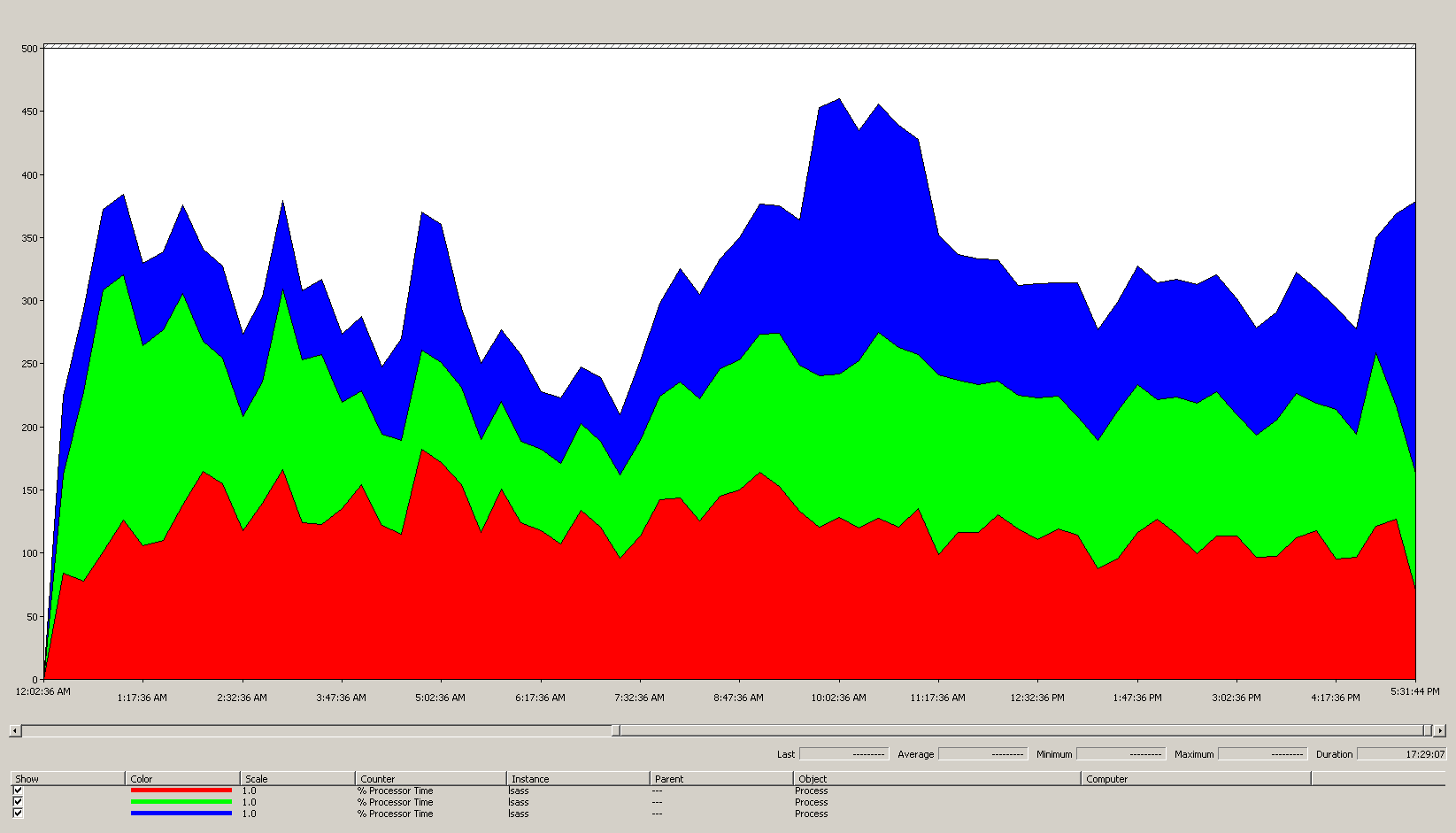
Here's what this chart tells us about the scenario environment:
- There are three domain controllers in the site.
- The business day starts ramping up around 7:00 AM, then ramps down at 5:00 PM.
- The busiest period of the day is from 9:30 AM to 11:00 AM.
Note
All performance data is historical. The peak data point at 9:15 AM indicates the load from 9:00 AM to 9:15 AM.
- Spikes before 7:00 AM could indicate extra load from different time zones or background infrastructure activity, such as backups. However, since this spike is lower than peak activity at 9:30 AM, it's not a cause for concern.
At maximum load, the lsass process consumes around 4.85 CPUs running at 100%, which would be 485% on a single CPU. These results suggest the scenario site needs about 12/25 CPUs to handle AD DS. When you bring in the recommended 5% to 10% extra capacity for background processes, the server needs 12.30 to 12.25 CPUs to support its current load. Estimates anticipating future growth make this number even higher.
When to tune LDAP weights
There are certain scenarios where you should consider tuning LdapSrvWeight. In the context of capacity planning, you'd tune it when your applications, user loads, or underlying system capabilities aren't evenly balanced.
The following sections describe two example scenarios where you should tune the Lightweight Directory Access Protocol (LDAP) weights.
Example 1: PDC emulator environment
If you're using a Primary Domain Controller (PDC) emulator, unevenly distributed user or application behavior can affect multiple environments at once. CPU resources on the PDC emulator are often more heavily demanded than elsewhere in the deployment because several tools and actions target it, such as Group Policy management tools, second authentication attempts, trust establishment, and so on.
- You should tune your PDC emulator only if there's a noticeable difference in CPU utilization. Tuning should reduce the load on the PDC emulator and increase the load on other DCs, allowing for more even load distribution.
- In these cases, set the value for
LDAPSrvWeightbetween 50 and 75 for the PDC emulator.
| System | CPU utilization with defaults | New LdapSrvWeight | Estimated new CPU utilization |
|---|---|---|---|
| DC 1 (PDC emulator) | 53% | 57 | 40% |
| DC 2 | 33% | 100 | 40% |
| DC 3 | 33% | 100 | 40% |
The catch is that if the PDC emulator role is transferred or seized, particularly to another domain controller in the site, then CPU utilization dramatically increase on the new PDC emulator.
In this example scenario, we assume based on Target site behavior profile that all three domain controllers in this site have four CPUs. Under normal conditions, what would happen if one of these DCs had eight CPUs? There would be two DCs at 40% utilization and one at 20% utilization. While this configuration isn't necessarily bad, there's an opportunity here for you to use LDAP weight tuning to balance the load better.
Example 2: environment with different CPU counts
When you have servers with different CPU counts and speeds in the same site, you need to make sure they're evenly distributed. For example, if your site has two eight-core servers and one four-core server, the four-core server only has half the processing power of the other two servers. If the client load is evenly distributed, that means the four-core server needs to work twice as hard as the two eight-core servers to manage its CPU load. On top of that, if one of the eight-core servers goes offline, the four-core server gets overloaded.
| System | Processor Information\ % Processor Utility(_Total) CPU utilization with defaults |
New LdapSrvWeight | Estimated new CPU utilization |
|---|---|---|---|
| 4-CPU DC 1 | 40 | 100 | 30% |
| 4-CPU DC 2 | 40 | 100 | 30% |
| 8-CPU DC 3 | 20 | 200 | 30% |
Planning for an “N + 1” scenario is of paramount importance. The impact of one DC going offline must be calculated for every scenario. In the immediately preceding scenario where the load distribution is even, in order to ensure a 60% load during an “N” scenario, with the load balanced evenly across all servers, the distribution is fine as the ratios stay consistent. When you look at the PDC emulator tuning scenario, or any general scenario where user or application load is unbalanced, the effect is very different:
| System | Tuned Utilization | New LdapSrvWeight | Estimated New Utilization |
|---|---|---|---|
| DC 1 (PDC emulator) | 40% | 85 | 47% |
| DC 2 | 40% | 100 | 53% |
| DC 3 | 40% | 100 | 53% |
Virtualization considerations for processing
When you're capacity planning for a virtualized environment, there are two levels you need to consider: the host level and the guest level. At the host level, you must identify the peak periods of your business cycle. Because scheduling guest threads on the CPU for a virtual machine is similar to getting AD DS threads on the CPU for a physical machine, we still recommend you use 40% to 60% of the underlying host. At the guest level, because the underlying thread scheduling principles are unchanged, we also still recommend you keep CPU usage within the 40% to 60% range.
In a direct-mapped scenario with one guest per host, you must bring in all capacity planning estimates you've done in the previous sections in order to make your estimate. For a shared host scenario, there's about 10% impact on the efficiency of the underlying processors, which means if a site needs 10 CPUs at a target of 40%, the recommended number of virtual CPUs you should allocate across all N guests would be 11. In sites with mixed distributions of physical and virtual servers, this modifier only applies to the virtual machines (VMs). For example, in an N + 1 scenario, one physical or direct-mapped server with 10 CPUs is almost equal to one guest with 11 CPUs on a host with 11 more CPUs reserved for the DC.
While you're analyzing and calculating how many CPUs you need to support AD DS load, keep in mind that if you plan to purchase physical hardware, the types of hardware available on the market may not map exactly to your estimates. However, you don't have that problem when you use virtualization. Using VMs decreases the effort needed for you to add compute capacity to a site, as you can add as many CPUs with the exact specifications you want to a VM. However, virtualization doesn't eliminate your responsibility to accurately evaluate how much compute power you need to guarantee your underlying hardware is available when guests need more CPU. As always, remember to plan ahead for growth.
Virtualization calculation summary example
| System | Peak CPU |
|---|---|
| DC 1 | 120% |
| DC 2 | 147% |
| DC 3 | 218% |
| Total CPU usage | 485% |
| Target system(s) count | Total bandwidth (from above) |
|---|---|
| CPUs needed at 40% target | 4.85 ÷ .4 = 12.25 |
When planning ahead for growth in this scenario, if you assume that demand will grow by 50% over the next three years, you need to make sure it has 18.375 CPUs (12.25 × 1.5) by that time. Alternatively, you can review demand after the first year, then add extra capacity based on what the results tell you.
Cross-trust client authentication load for NTLM
Evaluating cross-trust client authentication load
Many environments may have one or more domains connected by a trust. Authentication requests for identities in other domains that don't use Kerberos need to traverse a trust using a secure channel between two domain controllers. The domain controller the user is trying to access in the site connects to another domain controller that's located in either the destination domain or somewhere further up the path towards the destination domain. How many calls the DC can make to the other DC in the trusted domain is controlled by the *MaxConcurrentAPI setting. In order to ensure the secure channel can handle the amount of load required for the DCs to communicate with each other, you can either tune MaxConcurrentAPI or, if you're in a forest, create shortcut trusts. Learn more about how to determine traffic volume across trusts at How to do performance tuning for NTLM authentication by using the MaxConcurrentApi setting.
As with the previous scenarios, you must collect data during the peak busy periods of the day in order for it to be useful.
Note
Intraforest and interforest scenarios may cause the authentication to traverse multiple trusts, which means you need to tune during each stage of the process.
Virtualization planning
There are a few things you should keep in mind when capacity planning for virtualization:
- Many applications use Network Level Trust Manager (NTLM) authentication by default or in certain configurations.
- As the number of active clients increases, so does the need for application servers to have more capacity.
- Clients sometimes keep sessions open for a limited time and instead reconnect on a regular basis for services like email pull sync.
- Web proxy servers that require authentication for internet access can cause high NTLM load.
These applications can create a large load for NTLM authentication, which puts significant stress on the DCs, especially when users and resources are in different domains.
There are many approaches you can take to manage cross-trust load, which often you can and should use together at the same time:
- Reduce cross-trust client authentication by locating the services that a user consumes in the domain they're located in.
- Increase the number of secure channels available. These channels are called shortcut trusts and are relevant to intraforest and cross-forest traffic.
- Tune the default settings for MaxConcurrentAPI.
To tune MaxConcurrentAPI on an existing server, use the following equation:
New_MaxConcurrentApi_setting ≥ (semaphore_acquires + semaphore_time-outs) × average_semaphore_hold_time ÷ time_collection_length
For more information, see KB article 2688798: How to do performance tuning for NTLM authentication by using the MaxConcurrentApi setting.
Virtualization considerations
There aren't any special considerations you need to make, as virtualization is an operating system tuning setting.
Virtualization tuning calculation example
| Data type | Value |
|---|---|
| Semaphore Acquires (Minimum) | 6,161 |
| Semaphore Acquires (Maximum) | 6,762 |
| Semaphore Timeouts | 0 |
| Average Semaphore Hold Time | 0.012 |
| Collection Duration (seconds) | 1:11 minutes (71 seconds) |
| Formula (from KB 2688798) | ((6762 - 6161) + 0) × 0.012 / |
| Minimum value for MaxConcurrentAPI | ((6762 - 6161) + 0) × 0.012 ÷ 71 = .101 |
For this system for this time period, the default values are acceptable.
Monitoring for compliance with capacity planning goals
Throughout this article, we've discussed how planning and scaling go towards utilization targets. The following table summarizes the recommended thresholds you must monitor to ensure systems are operating as intended. Keep in mind that these aren't performance thresholds, just capacity planning thresholds. A server operating in excess of these thresholds will still work, but you need to validate your applications are working as intended before you start seeing performance issues as user demand increases. If the applications are okay, then you should start evaluating hardware upgrades or other configuration changes.
| Category | Performance counter | Interval/Sampling | Target | Warning |
|---|---|---|---|---|
| Processor | Processor Information(_Total)\% Processor Utility |
60 min | 40% | 60% |
| RAM (Windows Server 2008 R2 or earlier) | Memory\Available MB | < 100 MB | N/A | < 100 MB |
| RAM (Windows Server 2012) | Memory\Long-Term Average Standby Cache Lifetime(s) | 30 min | Must be tested | Must be tested |
| Network | Network Interface(*)\Bytes Sent/sec Network Interface(*)\Bytes Received/sec |
30 min | 40% | 60% |
| Storage | LogicalDisk((<NTDS Database Drive>))\Avg Disk sec/ReadLogicalDisk(( |
60 min | 10 ms | 15 ms |
| AD Services | Netlogon(*)\Average Semaphore Hold Time | 60 min | 0 | 1 second |
Appendix A: CPU sizing criteria
This appendix discusses useful terms and concepts that can help you estimate your environment's CPU sizing needs.
Definitions: CPU sizing
A processor (microprocessor) is a component that reads and executes program instructions.
A multi-core processor has multiple CPUs on the same integrated circuit.
A multi-CPU system has multiple CPUs that aren't on the same integrated circuit.
A logical processor is a processor that only has one logical computing engine from the perspective of the operating system.
These definitions include hyper-threaded, one core on multi-core processor, or a single core processor.
As today's server systems have multiple processors, multiple multi-core processors, and hyper-threading, these definitions are generalized to cover both scenarios. We use the term logical processor because it represents the OS and application perspective of the available computing engines.
Thread-level parallelism
Each thread is an independent task, as each thread has its own stack and instructions. AD DS is multi-threaded and you can tune the number of available threads by following the directions in How to view and set LDAP policy in Active Directory by using Ntdsutil.exe, it scales well across multiple logical processors.
Data-level parallelism
Data-level parallelism is when a service shares data across many threads for the same process and sharing many threads across multiple processes. The AD DS process alone would count as a service sharing data across several threads for a single process. Any changes to the data are reflected across all running threads in all levels of the cache, every core, and any updates to the shared memory. Performance can degrade during write operations because all memory locations adjust to the changes before instruction processing can continue.
CPU speed versus multiple-core considerations
Generally, faster logical processors reduce the time required to process a series of instructions. More logical processors mean you can run more tasks at the same time. However, these rules don't apply in scenarios that are more complex, such as fetching data from shared memory, waiting on data-level parallelism, and the overhead of managing multiple threads at once. As a result, scalability in multi-core systems isn't linear.
To understand why this change happens, it helps to think of these scenarios like a highway. Each thread is an individual car, each lane is a core, and the speed limit is the clock speed.
If there's only one car on the highway, it doesn't matter if there are two or 12 lanes. That car only goes as fast as the speed limit allows.
If the data the thread needs isn't immediately available, then the thread can't process instructions until it fetches the relevant data from memory. It's like if a segment of the highway is shut down. Even if there's only one car on the highway, the speed limit won't affect its ability to travel, because it can't go anywhere until the road is reopened.
As the number of cars increases, the overhead that the highway needs to manage the number of cars also increases. Drivers need to focus harder when driving on the highway during rush hour traffic as opposed to the late evening when the road is mostly empty. Also, driving on a two-lane highway where you only need to worry about one other lane requires less focus than driving on a six-lane highway where you have five other lanes of traffic to pay attention to.
In summary, questions about whether you should add more or faster processors become highly subjective and should be considered on a case-by-case basis. For AD DS in particular, its processing needs depend on environmental factors and can vary from server to server within a single environment. As a result, the earlier sections in this article didn't invest heavily on making super precise calculations. When you make budget-driven buying decisions, we recommend you first optimize processor usage at either 40% or whichever number your specific environment requires. If your system isn't optimized, then you don't benefit as much from buying additional processors.
Note
Amdahl's law and Gustafson's law are the relevant concepts here.
Response time and how system activity levels impact performance
Queuing theory is the mathematical study of waiting lines, or queues. In queuing theory for computing, the utilization law is represented by t equation:
U k = B ÷ T
Where U k is the utilization percentage, B is the amount of time spent being busy, and T is the total time spent observing the system. In a Microsoft context, this means the number of 100-nanosecond (ns) interval threads that are in a Running state divided by how many 100-ns intervals were available in the given time interval. This is the same formula that calculates percentage of processor utilization shown in Processor Object and PERF_100NSEC_TIMER_INV.
Queuing theory also provides the formula: N = U k ÷ (1 - U k) to estimate the number of waiting items based on utilization, where N is the length of the queue. Charting this equation over all utilization intervals provides the following estimates of how long the queue to get on the processor is at any given CPU load.
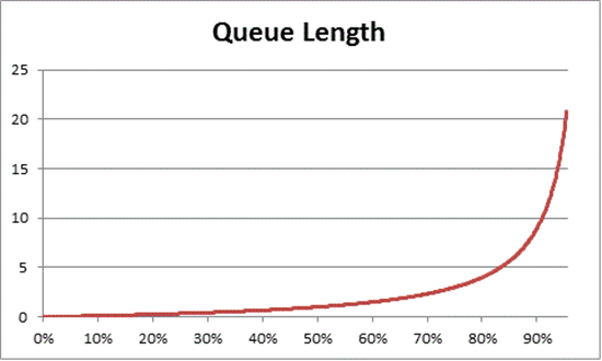
Based on this estimate, we can observe that after 50% CPU load, the average wait usually includes one other item in the queue, and increases rapidly to 70% CPU utilization.
To understand how queuing theory applies to your AD DS deployment, let's return to the highway metaphor we used in CPU speed versus multiple-core considerations.
Busier times in the mid-afternoon would fall somewhere into the 40% to 70% capacity range. There's enough traffic that your ability to choose a lane to drive in isn't severely restricted. While the chance of another driver getting in your way is high, it doesn't require the same level of effort you'd need to find a safe gap between other cars in the lane as during rush hour.
As rush hour approaches, the road system approaches 100% capacity. Changing lanes during rush hour becomes very challenging because cars are so close together that you don't have as much room to maneuver when changing lanes.
This is why estimating long term averages for capacity at 40% allows for more headroom for abnormal load spikes, whether those spikes are transitory, such as with poorly coded queries that take a while to run, or abnormal bursts in general load, like the spike in activity the morning after a holiday weekend.
The previous statement regards the percentage of processor time calculation as being the same as the utilization law equation. This simplified version is meant to introduce the concept to new users. However, for more advanced math, you can use the following references as a guide:
- Translating the PERF_100NSEC_TIMER_INV
- B = The number of 100-ns intervals that Idle thread spends on the logical processor. The change in the X variable in the PERF_100NSEC_TIMER_INV calculation
- T = the total number of 100-ns intervals in a given time range. The change in the Y variable in the PERF_100NSEC_TIMER_INV calculation.
- U k = The utilization percentage of the logical processor by the Idle Thread or % Idle Time.
- Working out the math:
- U k = 1 – %Processor Time
- %Processor Time = 1 – U k
- %Processor Time = 1 – B / T
- %Processor Time = 1 – X1 – X0 / Y1 – Y0
Applying these concepts to capacity planning
The math in the previous section probably makes determining how many logical processors you need in a system seem very complex. As a result, your approach to sizing the system should focus on determining maximum target utilization based on current load, then calculating the number of logical processors you need to reach that target. Furthermore, your estimate doesn't need to be perfectly exact. While logical processor speeds do have a significant impact on synchronization, performance can also be affected by other areas:
- Cache efficiency
- Memory coherence requirements
- Thread scheduling and synchronization
- Imperfectly balanced client loads
Since compute power is relatively low-cost, it's not worth investing too much time in calculating the perfectly exact number of CPUs you need.
It's also important to remember that the 40% recommendation, in this case, isn't a mandatory requirement. We use it as a reasonable start for making calculations. Different kinds of AD users need different levels of responsiveness. There may even be scenarios where environments can run at 80% or even 90% utilization at a sustained average without the increased wait times for processor access noticeably affecting client performance.
There are also other areas in the system that are much slower than the logical processor which you should also tune, including RAM access, disk access, and transmitting responses over the network. For example:
If you add processors to a system running at 90% utilization that's disk-bound, it probably won't significantly improve performance. If you look more closely at the system, there are lots of threads that aren't even getting onto the processor because they're waiting for I/O operations to complete.
Resolving disk-bound issues can mean that threads previously stuck in waiting state stop being stuck, creating more competition for CPU time. As a result, the 90% utilization will go to 100%. You need to tune both components in order to bring utilization back down to manageable levels.
Note
The
Processor Information(*)\% Processor Utilitycounter can exceed 100% with systems that have a Turbo mode. Turbo mode lets the CPU exceed the rated processor speed for short periods. If you need more information, look at the CPU manufacturers' documentation and counter descriptions.
Discussing whole-system utilization considerations also involves domain controllers as virtualized guests. Response time and how system activity levels impact performance applies to both host and guest in a virtualized scenario. In a host with only one guest, a DC or system has almost the same performance as it would on physical hardware. Adding more guests to the hosts increases the utilization of the underlying host, also increasing wait times to get access to the processors. Therefore, you must manage logical processor utilization at both host and guest levels.
Let's revisit the highway metaphor from the previous sections, only this time we're imagining the guest VM as an express bus. Express buses, as opposed to public transit or school buses, go straight to the rider's destination without making any stops.
Now, let's imagine four scenarios:
- A system's off-peak hours are like riding an express bus late at night. When the rider gets on, there are almost no other passengers and the road is nearly empty. Because there's no traffic for the bus to contend with, the ride is easy and just as fast as if the rider had driven there in their own car. However, the rider's travel time is also constrained by the local speed limit.
- Off-peak hours when a system's CPU utilization is too high is like a late night ride when most of the lanes on the highway are closed. Even though the bus itself is mostly empty, the road is still congested from leftover traffic dealing with the restricted lanes. While the rider is free to sit anywhere they want, their actual trip time is determined by the traffic outside of the bus.
- A system with high CPU utilization during peak hours is like a crowded bus during rush hour. Not only does the trip take longer, but getting on and off the bus is harder because the bus is full of other passengers. Adding more logical processors to the guest system to try to speed up wait times would be like trying to solve the traffic problem by adding more buses. The problem isn't the number of buses, but how long the trip takes.
- A system with high CPU utilization during off-peak hours is like that same crowded bus on a mostly empty road at night. While riders may have trouble finding seats or getting on and off the bus, the trip is fairly smooth once the bus picks up all its passengers. This scenario is the only one where performance would improve by adding more buses.
Based on the previous examples, you can see that there are many scenarios between 0% and 100% utilization that have varying degrees of impact on performance. Also, adding more logical processors doesn't necessarily improve performance outside of very specific scenarios. It should be fairly simple to apply these principles to the recommended 40% CPU utilization target for hosts and guests.
Appendix B: Considerations regarding different processor speeds
In Processing, we assumed that the processor is running at 100% clock speed while you collect data, and that any replacement systems have the same processing speed. Despite these assumptions not being accurate, especially for Windows Server 2008 R2 and later, where the default power plan is Balanced, these assumptions still work for conservative estimates. While potential errors may increase, it only increases the margin of safety as processor speeds increase.
- For example, in a scenario that demands 11.25 CPUs, if the processors ran at half speed when you collected your data, the more accurate estimate of their demand would be 5.125 ÷ 2.
- It's impossible to guarantee that doubling clock speed doubles the amount of processing that happens within the recorded time period. The amount of time that processors spend waiting on RAM or other components stays roughly the same. Therefore, faster processors might spend a greater percentage of time idle while waiting for the system to fetch data. We recommend you stick with the lowest common denominator, keep your estimates conservative, and avoid assuming a linear comparison between processor speeds that could make your results inaccurate.
If processor speeds in your replacement hardware are lower than your current hardware, you should proportionally increase the estimate of how many processors you need. For example, let's look at a scenario where you calculate you need 10 processors to sustain your site's load. The current processors run at 3.3 GHz, and the processors you plan to replace them with run at 2.6 GHz. Replacing only the 10 original processors would give you a 21% decrease in speed. To increase speed, you need to get at least 12 processors instead of 10.
However, this variability doesn't change capacity management processor utilization targets. Processor clock speeds adjust dynamically based on load demand, so running the system under higher loads causes the CPU to spend more time in a higher clock speed state. The ultimate goal is to have the CPU be at 40% utilization in a 100% clock speed state during peak business hours. Anything less will generate power savings by throttling CPU speeds during off-peak scenarios.
Note
You can turn off power management on the processors during data collection by setting the power plan to High Performance. Turning power management off gives you more accurate readings of CPU consumption in the target server.
To adjust estimates for different processors, we recommend you use the SPECint_rate2006 benchmark from Standard Performance Evaluation Corporation. To use this benchmark:
Go to the Standard Performance Evaluation Corporation (SPEC) website.
Select Results.
Enter CPU2006 and select Search.
In the drop-down menu for Available Configurations, select All SPEC CPU2006.
In the Search Form Request field, select Simple, then select Go!.
Under Simple Request, enter the search criteria for your target processor. For example, if you're looking for an ES-2630 processor, in the drop-down menu, select Processor, then enter the processor name in the search field. When finished, select Execute Simple Fetch.
Look for your server and processor configuration in the search results. If the search engine doesn't return an exact match, look for the closest match possible.
Record the values in the Result and # Cores columns.
Determine the modifier by using this equation:
((Target platform per-core score value) × (MHz per-core of baseline platform)) ÷ ((Baseline per-core score value) × (MHz per-core of target platform))
For example, here's how you'd find the modifier for an ES-2630 processor:
(35.83 × 2000) ÷ (33.75 × 2300) = 0.92
Multiply the number of processors you estimate you need by this modifier.
For the ES-2630 processor example, 0.92 × 10.3 = 10.35 processors.
Appendix C: How the operating system interacts with storage
The queuing theory concepts we discussed in Response time and how system activity levels impact performance also apply to storage. You need to be familiar with how your OS handles I/O in order to apply these concepts effectively. In Windows OSes, the OS creates a queue that holds I/O requests for each physical disk. However, a physical disk isn't necessarily a single disk. The OS can also register an aggregation of spindles on an array controller or SAN as a physical disk. Array controllers and SANs can also aggregate multiple disks into a single array set, split it into multiple partitions, then use each partition as a physical disk, as shown in the following image.
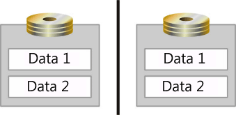
In this illustration, the two spindles are mirrored and split into logical areas for data storage, labeled Data 1 and Data 2. The OS registers each of these logical areas as separate physical disks.
Now that we've clarified what defines a physical disk, you should also get familiar with the following terms to help you better understand the information in this Appendix.
- A spindle is the device physically installed in the server.
- An array is a collection of spindles aggregated by the controller.
- An array partition is a partitioning of the aggregated array.
- A Logical Unit Number (LUN) is an array of SCSI devices connected to a computer. This article uses these terms when talking about SANs.
- A disk includes any spindle or partition that the OS registers as a single physical disk.
- A partition is a logical partitioning of what the OS registers as a physical disk.
Operating system architecture considerations
The OS creates a First In, First Out (FIFO) I/O queue for each disk it registers. These disks can be spindles, arrays, or array partitions. When it comes to how the OS handles I/O, the more active queues, the better. When the OS serializes the FIFO queue, it must process all FIFO I/O requests issued to the storage subsystem in order of arrival. When the OS correlates each disk with a spindle or array, it maintains an I/O queue for each unique set of disks, eliminating competition for scarce I/O resources across disks and isolating I/O demand to a single disk. However, Windows Server 2008 introduced an exception in the form of I/O prioritization. Applications designed to use low priority I/O are moved to the back of the queue no matter when the OS received them. Applications not specifically coded to use the low priority setting default to normal priority instead.
Introducing simple storage subsystems
In this section, we talk about simple storage subsystems. Let's start with an example: a single hard drive inside a computer. If we break down this system into its major storage subsystem components, here's what we get:
- One 10,000 RPM Ultra Fast SCSI HD (Ultra Fast SCSI has a 20 MBps transfer rate)
- One SCSI Bus (the cable)
- One Ultra Fast SCSI Adapter
- One 32-bit 33 MHz PCI bus
Note
This example doesn't reflect the disk cache where the system typically keeps the data of one cylinder. In this case, the first I/O needs 10 ms and the disk reads the whole cylinder. All other sequential I/Os are satisfied by the cache. As a result, in-disk caches might improve sequential I/O performance.
Once you identify the components, you can begin to get an idea of how much data the system can transmit and how much I/O it can handle. The amount of I/O and quantity of data that can transit the system are related to each other, but not the same value. This correlation depends on the block size and whether the disk I/O is random or sequential. The system writes all data to the disk as a block, but different applications can use different block sizes.
Next, let's analyze these items on a component-by-component basis.
Hard drive access times
The average 10,000-RPM hard drive has a 7 ms seek time and a 3 ms access time. Seek time is the average amount of time it takes the read or write head to move to a location on the platter. Access time is the average amount of time it takes for the head to read or write the data to disk once it's in the correct location. Therefore, the average time for reading a unique block of data in a 10,000-RPM HD includes both seek and access times for a total of approximately 10 ms, or .010 seconds, per block of data.
When every disk access requires the head move to a new location on the disk, the read or write behavior is called random. When all I/O is random, a 10,000-RPM HD can handle approximately 100 I/O per second (IOPS).
When all I/O occurs from adjacent sectors on the hard drive, we call it sequential I/O. Sequential I/O has no seek time because, after the first I/O finishes, the read or write head is at the start of where the hard drive is storing the next data block. For example, a 10,000-RPM HD is capable of handling approximately 333 I/O per second, based on the following equation:
1000 ms per second ÷ 3 ms per I/O
So far, the transfer rate of the hard drive hasn't been relevant to our example. No matter the hard drive size, the actual amount of IOPS the 10,000-RPM HD can handle is always about 100 random or 300 sequential I/Os. As block sizes change based on which application is writing to the drive, the amount of data pulled per I/O also changes. For example, if the block size is 8 KB, 100 I/O operations will read from or write to the hard drive a total of 800 KB. However, if the block size is 32 KB, 100 I/O will read or write 3,200 KB (3.2 MB) to the hard drive. If the SCSI transfer rate exceeds the total amount of transferred data, then getting a faster transfer rate doesn't change anything. For more information, see the following tables:
| Description | 7200 RPM 9 ms seek, 4 ms access | 10,000 RPM 7 ms seek, 3 ms access | 15,000 RPM 4 ms seek, 2 ms access |
|---|---|---|---|
| Random I/O | 80 | 100 | 150 |
| Sequential I/O | 250 | 300 | 500 |
| 10,000 RPM drive | 8 KB block size (Active Directory Jet) |
|---|---|
| Random I/O | 800 KB/s |
| Sequential I/O | 2400 KB/s |
The SCSI backplane
How the SCSI backplane, which in this example scenario is the ribbon cable, impacts throughput of the storage subsystem depends on block size. How much I/O can the bus handle if the I/O is in 8 KB blocks? In this scenario, the SCSI bus is 20 MBps, or 20480 KB/s. 20480 KB/s divided by 8 KB blocks yields a maximum of approximately 2500 IOPS supported by the SCSI bus.
Note
The figures in the following table represent an example scenario. Most attached storage devices currently use PCI Express, which provides much higher throughput.
| I/O supported by SCSI bus per block size | 2 KB block size | 8 KB block size (AD Jet) (SQL Server 7.0/SQL Server 2000) |
|---|---|---|
| 20 MBps | 10,000 | 2,500 |
| 40 MBps | 20,000 | 5,000 |
| 128 MBps | 65,536 | 16,384 |
| 320 MBps | 160,000 | 40,000 |
As the previous table shows, in our example scenario, the bus is never a bottleneck because the spindle maximum is 100 I/O, way below any of the listed thresholds.
Note
In this scenario, we're assuming that the SCSI bus is 100% efficient.
The SCSI adapter
In order to determine how much I/O the system can handle, you must check the manufacturer's specifications. Directing I/O requests to the appropriate device requires processing power, so how much I/O the system can handle depends on the SCSI adaptor or array controller processor.
In this example scenario, we're assuming that the system can handle 1,000 I/O.
The PCI bus
The PCI bus is an oft-overlooked component. In this example scenario, the PCI bus isn't the bottleneck. However, as systems scale up, it can potentially become a bottleneck in the future.
We can see how much a PCI bus can transfer data in our example scenario by using this equation:
32 bits ÷ 8 bits per byte × 33 MHz = 133 MBps
Therefore, we can assume a 32 bit PCI bus operating at 33 Mhz can transfer 133 MBps of data.
Note
This equation's result represents the theoretical limit of transferred data. In reality, most systems only reach about 50% of maximum limit. In certain burst scenarios, the system can reach 75% of the limit for short periods.
A 66 MHz 64-bit PCI bus can support a theoretical maximum of 528 MBps based on this equation:
64 bits ÷ 8 bits per byte × 66 Mhz = 528 MBps
When you add any other device, such as a network adapter or a second SCSI controller, it reduces bandwidth available to the system, as all devices share the bandwidth and can compete with each other for limited processing resources.
Analyzing storage subsystems to find bottlenecks
In this scenario, the spindle is the limiting factor for how much I/O you can request. As a result, this bottleneck also limits how much data the system can transmit. Because our example is an AD DS scenario, the amount of transmittable data is 100 random I/O per second in 8 KB increments, for a total of 800 KB per second when you access the Jet database. In contrast, the maximum throughput for a spindle you configure to exclusively allocate to log files would be limited to 300 sequential I/O per second in 8 KB installments, totaling at 2,400 KB or 2.4 MB per second.
Now that we've analyzed the components of our example configuration, let's look at a table that demonstrates where bottlenecks can happen as we add and change components in the storage subsystem.
| Notes | Bottleneck analysis | Disk | Bus | Adapter | PCI bus |
|---|---|---|---|---|---|
| This is the domain controller configuration after adding a second disk. The disk configuration represents the bottleneck at 800 KB/s. | Add 1 disk (Total=2) I/O is random 4 KB block size 10,000 RPM HD |
200 I/Os total 800 KB/s total. |
|||
| After adding 7 disks, the disk configuration still represents the bottleneck at 3200 KB/s. | Add 7 disks (Total=8) I/O is random 4 KB block size 10,000 RPM HD |
800 I/Os total. 3200 KB/s total |
|||
| After changing I/O to sequential, the network adapter becomes the bottleneck because it's limited to 1000 IOPS. | Add 7 disks (Total=8) I/O is sequential 4 KB block size 10,000 RPM HD |
2400 I/O sec can be read/written to disk, controller limited to 1000 IOPS | |||
| After replacing the network adapter with a SCSI adapter that supports 10,000 IOPS, the bottleneck returns to the disk configuration. | Add 7 disks (Total=8) I/O is random 4 KB block size 10,000 RPM HD Upgrade SCSI adapter (now supports 10,000 I/O) |
800 I/Os total. 3,200 KB/s total |
|||
| After increasing the block size to 32 KB, the bus becomes the bottleneck because it only supports 20 MBps. | Add 7 disks (Total=8) I/O is random 32 KB block size 10,000 RPM HD |
800 I/Os total. 25,600 KB/s (25 MBps) can be read/written to disk. The bus only supports 20 MBps |
|||
| After upgrading the bus and adding more disks, the disk remains the bottleneck. | Add 13 disks (Total=14) Add second SCSI adapter with 14 disks I/O is random 4 KB block size 10,000 RPM HD Upgrade to 320 MBps SCSI bus |
2800 I/Os 11,200 KB/s (10.9 MBps) |
|||
| After changing I/O to sequential, the disk remains the bottleneck. | Add 13 disks (Total=14) Add second SCSI Adapter with 14 disks I/O is sequential 4 KB block size 10,000 RPM HD Upgrade to 320 MBps SCSI bus |
8,400 I/Os 33,600 KB\s (32.8 MB\s) |
|||
| After adding faster hard drives, the disk remains the bottleneck. | Add 13 disks (Total=14) Add second SCSI adapter with 14 disks I/O is sequential 4 KB block size 15,000 RPM HD Upgrade to 320 MBps SCSI bus |
14,000 I/Os 56,000 KB/s (54.7 MBps) |
|||
| After increasing the block size to 32 KB, the PCI bus becomes the bottleneck. | Add 13 disks (Total=14) Add second SCSI adapter with 14 disks I/O is sequential 32 KB block size 15,000 RPM HD Upgrade to 320 MBps SCSI bus |
14,000 I/Os 448,000 KB/s (437 MBps) is the read/write limit to the spindle. The PCI bus supports a theoretical maximum of 133 MBps (75% efficient at best). |
Introducing RAID
When you introduce an array controller to your storage subsystem, it doesn't dramatically change its nature. The array controller only replaces the SCSI adapter in the calculations. However, the cost of reading and writing data to the disk when you use the various array levels does change.
In RAID 0, writing data stripes it across all disks in the RAID set. During a read or write operation, the system pulls data from or pushes it to each disk, increasing the amount of data the system can transmit during this particular time period. Therefore, in this example where we're using 10,000 RPM drives, using RAID 0 would let you perform 100 I/O operations. The total amount of I/O the system supports is N spindles times 100 1/O per second per spindle, or N spindles × 100 I/O per second per spindle.

In RAID 1, the system mirrors, or duplicates, data across a pair of spindles for redundancy. When the system performs a read I/O operation, it can read data from both spindles in the set. This mirroring makes I/O capacity for both disks available during a read operation. However, RAID 1 doesn't give write operations any performance advantages, because the system also needs to mirror written data on the pair of spindles. Although mirroring doesn't make write operations take longer, it does prevent the system from making more than one read operation at the same time. Therefore, every write I/O operation costs two read I/O operations.
The following equation calculates how many I/O operations are happening in this scenario:
Read I/O + 2 × Write I/O = Total available disk I/O consumed
When you know the ratio of reads to writes and the number of spindles in your deployment, you can use this equation to calculate how much I/O your array can support:
Maximum IOPS per spindle × 2 spindles × [(% Reads + % Writes) ÷ (% Reads + 2 × % Writes)] = Total IOPS
A scenario using both RAID 1 and RAID 0 behaves exactly like RAID 1 in the cost of reading and writing operations. However, the I/O is now striped across each mirrored set. This means the equation will change to this:
Maximum IOPS per spindle × 2 spindles × [(% Reads + % Writes) ÷ (% Reads + 2 × % Writes)] = Total I/O
In a RAID 1 set, when you stripe N number of RAID 1 sets, the total I/O your array can process becomes N × I/O per RAID 1 set:
N × {Maximum IOPS per spindle × 2 spindles × [(% Reads + % Writes) ÷ (% Reads + 2 × % Writes)]} = Total IOPS
We sometimes call RAID 5 N + 1 RAID because the system stripes the data across N spindles and writes parity information to the + 1 spindle. However, RAID 5 uses more resources when performing a write I/O than RAID 1 or RAID 1 + 0. RAID 5 performs the following process every time the operating system submits a write I/O to the array:
- Read the old data.
- Read the old parity.
- Write the new data.
- Write the new parity.
Every write I/O request that the OS sends to the array controller requires four I/O operations to finish. Therefore, N + 1 RAID write requests take four times as long as a read I/O to finish. In other words, to determine how many I/O requests from the OS translate to how many requests the spindles get, you use this equation:
Read I/O + 4 × Write I/O = Total I/O
Similarly, in a RAID 1 set where you know the ratio of reads to writes and how many spindles there are, you can use this equation to identify how much I/O your array can support:
IOPS per spindle × (Spindles – 1) × [(% Reads + % Writes) ÷ (% Reads + 4 × % Writes)] = Total IOPS
Note
The previous equation's result doesn't include the drive lost to parity.
Introducing SANs
When you introduce a storage area network (SAN) into your environment, it doesn't affect the planning principles we've described in the earlier sections. However, you should take into account that the SAN can change the I/O behavior for all systems connected to it. One of the main advantages of using a SAN is that it gives you more redundancy over internally or externally attached storage, but it also means your capacity planing needs to account for fault tolerance needs. Also, as you introduce more components to your system, you also need to factor these new parts into your calculations.
Now, let's break down a SAN into its components:
- The SCSI or Fibre Channel hard drive
- The storage unit channel backplane
- The storage units themselves
- The storage controller module
- One or more SAN switches
- One or more host bus adapters (HBAs)
- The peripheral component interconnect (PCI) bus
When you design a system for redundancy, you must include extra components to ensure your system keeps working during a crisis scenario where one or more of the original components stop working. However, when you're capacity planning, you need to exclude redundant components from available resources to get an accurate estimate of your system's baseline capacity, as those components don't usually come online unless there's an emergency. For example, if your SAN has two controller modules, you only need to use one when calculating total available I/O throughput, as the other won't turn on unless the original module stops working. You also shouldn't bring the redundant SAN switch, storage unit, or spindles into I/O calculations.
Also, because your capacity planning only considers periods of peak usage, you shouldn't factor redundant components into your available resources. Peak utilization shouldn't exceed 80% saturation of the system in order to accommodate bursts or other unusual system behavior.
When you analyze the behavior of the SCSI or Fibre Channel hard drive, you should analyze it according to the principles we outlined in previous sections. Despite each protocol having their own advantages and disadvantages, the main thing that limits performance on a per-disk basis is the mechanical limitations of the hard drive.
When you analyze the channel on the storage unit, you should take the same approach you did when calculating how many resources were available on the SCSI bus: divide the bandwidth by the block size. For example, if your storage unit has six channels that each support a 20 MBps maximum transfer rate, your total amount of available I/O and data transfer is 100 MBps. The reason the total is 100 MBps instead of 120 MBps is because the storage channel total throughput shouldn't exceed the amount of throughput it would use if one of the channels suddenly turned off, leaving it with only five functioning channels. Of course, this example also assumes that the system is evenly distributing load and fault tolerance across all channels.
Whether you can turn the previous example into an I/O profile depends on the application behavior. For Active Directory Jet I/O, the maximum value would be approximately 12,500 I/O per second, or 100 MBps ÷ 8 KB per I/O.
In order to understand how much throughput your controller modules support, you also need to get their manufacturer specifications. In this example, the SAN has two controller modules that support 7,500 I/O each. If you aren't using redundancy, then the total system throughput would be 15,000 IOPS. However, in a scenario where redundancy is required, you'd calculate the maximum throughput based on the limits of only one of the controllers, which is 7,500 IOPS. Assuming that the block size is 4 KB, this threshold is well below the 12,500 IOPS maximum that the storage channels can support, and is therefore the bottleneck in your analysis. However, for planning purposes, the desired maximum I/O you should plan for is 10,400 I/O.
When the data leaves the controller module, it transmits a Fibre Channel connection rated at 1 GBps, or 128 MBps. Because this amount exceeds the total bandwidth of 100 MBps across all the storage unit channels, it won't bottleneck the system. Also, because this transmission is on only one of the two Fibre Channels due to redundancy, if one Fibre Channel connection stops working, the remaining connection still has enough capacity to handle the data transfer demand.
The data then transits a SAN switch on its way to the server. The switch limits the amount of I/O it can handle because it needs to process the incoming request and then forward it to the appropriate port. However, you can only know what the switch limit is if you look at the manufacturer specifications. For example, if your system has two switches and each switch can handle 10,000 IOPS, the total throughput will be 20,000 IOPS. Based on the rules of fault tolerance, if one switch stops working, the total system throughput will be 10,000 IOPS. Therefore, during normal circumstances, you shouldn't use more than 80% utilization, or 8,000 I/O.
Finally, the HBA you install in the server also limits how much I/O it can handle. Typically, you install a second HBA for redundancy, but like with the SAN switch, when you calculate how much I/O the system can handle, the total throughput will be N - 1 HBA.
Caching considerations
Caches are one of the components that can significantly impact overall performance anywhere in the storage system. However, a detailed analysis of caching algorithms is beyond the scope of this article. Instead, we'll give you a quick list of things you should know about caching on disk subsystems.
- Caching improves sustained sequential write I/O because it buffers many smaller write operations into larger I/O blocks. It also destages operations to storage in a few big blocks instead of many tiny ones. This optimization reduces total random and sequential I/O operations, making more resources available for other I/O operations.
- Caching doesn't improve sustained write I/O throughput on the storage subsystem because it only buffers writes until spindles are available to commit the data. When all available I/O from the spindles is saturated by data for long periods of time, then the cache eventually fills up. To empty the cache, you must provide enough I/O for the cache to clear itself by providing extra spindles or giving enough time between bursts for the system to catch up.
- Larger caches allow for more data to buffer, which means the cache can handle longer periods of saturation.
- In typical storage subsystems, the OS experiences improved write performance with caches, as the system only needs to write the data to the cache. However, once the underlying media is saturated with I/O operations, the cache fills up and write performance returns to regular disk speed.
- When you cache read I/O, the cache is most useful when you store data sequentially on the desk and allow the cache to read ahead. Reading ahead is when the cache can immediately move to the next sector as if the next sector contains the data the system will request next.
- When read I/O is random, caching at the drive controller doesn't increase how much data the disk can read. If the OS or application-based cache size is bigger than the hardware-based cache size, then any attempts to enhance the disk read speed don't change anything.
- In Active Directory, the cache is only limited by the amount of RAM the system holds.
SSD considerations
Solid state drives (SSDs) are fundamentally different than spindle-based hard disks. SSDs can handle higher volumes of I/O with lower latency. While SSDs can be expensive on a cost-per-Gigabyte basis, they're very cheap in terms of cost-per-I/O. However, capacity planning with SSDs involves asking yourself the same questions that you would ask about spindles: how many IOPS can they handle and and what is the latency of those IOPS?
Here are some things you should consider when planning for SSDs:
- Both IOPS and latency are subject to manufacturer designs. In some cases, certain SSD designs can perform worse than spindle-based technologies. When trying to decide whether you should use SSD or spindles, you should review and validate manufacturer specs drive by drive instead of assuming all technologies work a certain way.
- IOPS types can have different values depending on whether they're read or write. AD DS services are predominantly read-based, and therefore are less effected by which write technology you use compare dto other application scenarios.
- Write endurance is the assumption that SSD cells have a limited lifespan and will eventually wear out after you use them a lot. For database drives, a predominantly read I/O profile extends the write endurance of cells to the point where you don't need to worry about write endurance that much.
Summary
Imagine storage as being like a house's indoor plumbing. The IOPS of the media you store your data in is like the home's main drain. When the main drain gets clogged or limited by size or pipe collapse, then the drains back up and don't work properly when the household uses a lot of water. This scenario is like when a shared environment has one or more systems using shared storage on the same SAN, NAS, or iSCSI with the same underlying media. Because user demand exceeds the system's ability to keep up, performance suffers.
Likewise, in our imaginary plumbing scenario, you can take different approaches to resolve clogs and other performance issues:
- To address a collapsed drain pipe or a drain that's too small, you need to replace the pipes with working and correctly sized ones. In shared storage terms, it's like adding new hardware or redistributing usage on the shared systems throughout the infrastructure.
- Unclogging a drain requires identifying the underlying problems and their locations, then removing them with the appropriate tool. For example, a relatively simple clog in a kitchen sink drain only needs a plunger or drain cleaner to remove, while more complex clogs that involve a trapped object may require a drain snake. Likewise, in a shared storage system, identifying the cause of performance issues helps you figure you out whether you need to create a system-level backup, synchronize antivirus scans across all servers, or synchronize the defragmentation software you run during peak periods.
In most plumbing designs, multiple drains feed into the main drain. When a drain gets clogged, water only gets trapped behind the point where the clog is. If a junction gets clogged, then all the drains behind that junction point stop draining. In a storage scenario, a junction getting clogged is like an overloaded switch, a driver compatibility issue, or unsynchronized software tasks. You must measure the IOPS and I/O size to determine whether your storage system can handle the load, then adjust the system as needed.
Appendix D: storage troubleshooting in environments where more RAM isn't an option
Many storage recommendations before virtualized storage served two purposes:
- Isolating I/O to prevent performance issues on the OS spindle from impacting performance for the database and I/O profiles.
- Taking advantage of the performance boost that spindle-based hard drives and caches can give your system when used with the sequential I/O of AD DS log files. Isolating sequential I/O to a separate physical drive can also increase throughput.
With new storage options, a lot fundamental assumptions behind earlier storage recommendations are no longer true. Virtualized storage scenarios, such as iSCSI, SAN, NAS, and Virtual Disk image files, often share underlying storage media across multiple hosts. This difference negates the assumptions that you must isolate I/O and optimize sequential I/O. Now other hosts that access the shared media can reduce responsiveness to the domain controller.
When you capacity plan for storage performance, you should consider three things:
- Cold cache state
- Warm cache state
- Backup and restore
The cold cache state is when you initially reboot the domain controller or restart the Active Directory service, so there's no Active Directory data in the RAM. A warm cache state is when the domain controller is operating in a steady state and has cached the database. In terms of performance design, warming a cold cache is like a sprint, while running a server with a fully warmed cache is like a marathon. Defining these states and the different performance profiles they drive is important, as you need to consider them both when estimating capacity. For example, just because you have enough RAM to cache the entire database during a warm cache state doesn't help you optimize performance during cold cache state.
For both cache scenarios, the most important thing is how fast storage can move data from disk to memory. When you warm the cache, over time performance improves as queries reuse data, the cache hit rate increases, and the frequency of going to the disk to retrieve data decreases. As a result, adverse performance impacts from having to go to the disk also decrease. Any performance degradations are temporary and usually go away when the cache reaches its warm state and the maximum size the system allows.
You can measure how quickly the system can get data from the disk by measuring the available IOPS in Active Directory. How many available IOPS there are is also subject to how many IOPS are available in the underlying storage. From a planning perspective, because warming the cache and backup or restore states are exceptional events that usually occur off peak hours and are subject to DC load, we can't give general recommendations beyond only entering these states during off-peak hours.
In most scenarios, AD DS is predominantly read I/O with a ratio of 90% read to 10% write. Read I/O is the typical bottleneck for user experience, while write I/O is the bottleneck that degrades write performance. Caches tend to provide minimal benefit to read I/O because I/O operations for the NTDS.dit file are predominantly random. Therefore, your main priority is to make sure you correctly configure the read I/O profile storage.
Under normal operating conditions, your storage planning goal is to minimize wait times for the system to return requests from AD DS to the disk. The number of outstanding and pending I/O operations should be less than or equal to the number of pathways in the disk. For performance monitoring scenarios, we generally recommend that the LogicalDisk((<NTDS Database Drive>))\Avg Disk sec/Read counter should be less than 20 ms. You should set the operating threshold much lower, as close to the speed of storage as possible, within a range of two to six milliseconds depending on the type of storage.
The following line graph shows the disk latency measurement within a storage system.
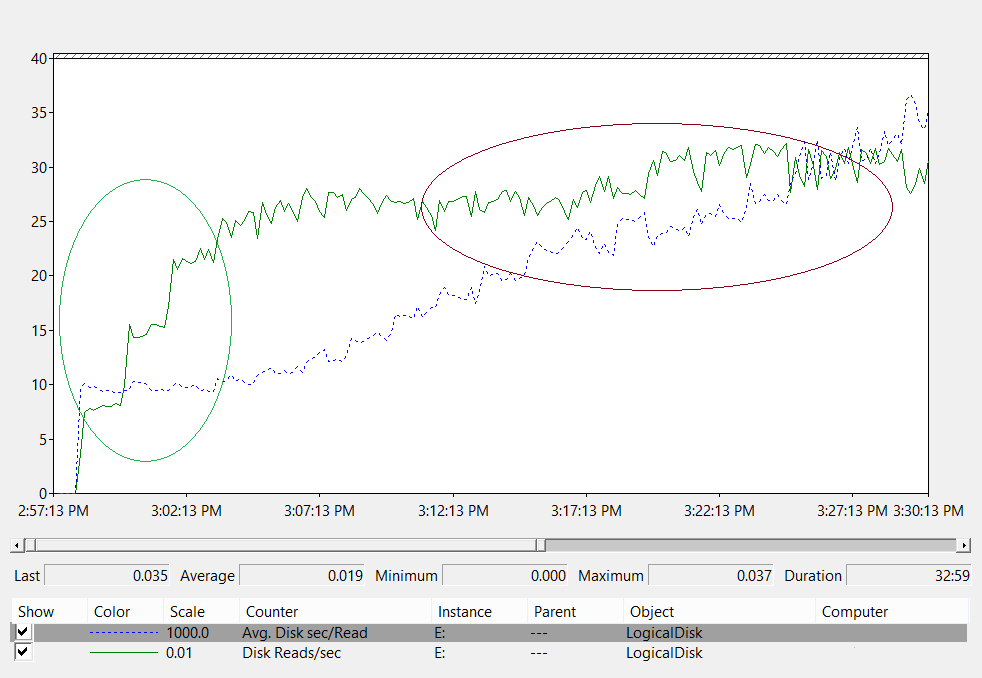
Let's analyze this line graph:
- The area on the left of the chart that's circled in green shows the latency is consistent at 10 ms as the load increases from 800 IOPS to 2,400 IOPS. This area is the baseline for how quickly the underlying storage can process an I/O request. However, this baseline is affected by what kind of storage solution you use.
- The area on the right side of the chart circled in maroon shows the system throughput between the baseline and the end of data collection. The throughput itself doesn't change, but the latency increases. This area demonstrates how requests spend a longer time waiting in the queue to be sent to the storage subsystem whenever request volumes exceed the physical limits of the underlying storage.
Now, let's think about what this data tells us.
First, let's assume a user querying membership of a large group requires the system read 1 MB of data from the disk. You can evaluate the amount of I/O required and how long the operations will take with these values:
- The size of each Active Directory database page is 8 KB.
- The minimum number of pages the system needs to read is 128.
- Therefore, at the baseline area in the diagram, the system should take at least 1.28 seconds to load the data from the disk and return it to the client. At the 20 ms mark, where the throughput goes well above the recommended maximum, the process takes 2.5 seconds.
Based on those numbers, you can calculate how fast the cache will warm by using this equation:
2,400 IOPS × 8 KB per I/O
After running this calculation, we can say that the cache warm rate in this scenario is 20 MBps. In other words, the system loads about 1 GB of database into the RAM every 53 seconds.
Note
It's normal to see latency go up for short periods while components are aggressively reading or writing to the disk. For example, latency increases when the system is backing up or AD DS runs garbage collection. You should provide additional room for these periodic events on top of your original usage estimates. Your goal is to give enough throughput to accommodate these spikes without affecting overall functioning.
There's a physical limit to how quickly the cache warms based on how you design the storage system. The only thing that can warm the cache up to the rate the underlying storage can accommodate are incoming client requests. Running scripts to try to pre-warm the cache during peak hours competes with real client requests, increases overall load, loads data that's not relevant to client requests, and degrades performance. We recommend you avoid using artificial measures to warm the cache.