Building a Finite Element Based Physics Engine - Continuum Mechanics
This article is the second in a five part series on generating the realistic synthetic motion of objects through finite elements techniques, culminating in the development of a physics engine.
- Introduction and Background
- Continuum Mechanics
- The Finite Element Model
- Code Implementation (Maya)
- Plasticity and Fracture
CONTINUUM MECHANICS
The field of continuum mechanics is a branch of engineering where a material, body or object is considered to have a continuous distribution of constitutive properties. Such a statement appears to be counter-intuitive given that, from an early age, we are taught that all matter is inherently discontinuous, composed of building blocks at the atomic scale such as nuclei and electrons.
Perhaps a better description would be to consider a continuum as the smallest possible quantity of a material (from both a physical and temporal sense) that can be analysed without having to take into account molecular dynamics or quantum mechanics. This assumption is further validated by considering that all interesting physical phenomena worthy of computer animation take place at lengths much greater than atomic spacing’s (10−10m) and over time periods far larger than atomic bond vibrations (10−15sec).
The discipline unites solid and fluid mechanics into one flexible theory that is concerned with the deformation of a material in response to external loading. For the purposes of this project, solid mechanics is of most interest and can be further subdivided into categories of elasticity and plasticity based on whether or not a material returns to its initial configuration when external forces are removed. Given that all materials must conserve mass, momentum and energy - it is the constitutive relationship between loading and deformation (stress and strain) that distinguishes different types of materials and governs their resulting behaviour.
STRESS AND STRAIN
Stress ( σ ) refers to the intensity of forces induced by a load on a material, often characterised as the force per unit area, while strain is the resulting deformation. Consider the general one-dimensional case of a rod with initial length L that is elongated to length L0 (in the x-direction only) due to the application of an external force. The dimensionless ratio of normal strain () can be considered as the change in length per unit original length and is defined mathematically in the equation below. Such an example is synonymous with an elastic spring but for materials of interest to computer animation, stress and strain will not be uniform from point to point.

Instead further refinement is required by introducing the displacement field u(x) = x0 − x. Consider the segment [xi,xj] shown in the figure below.
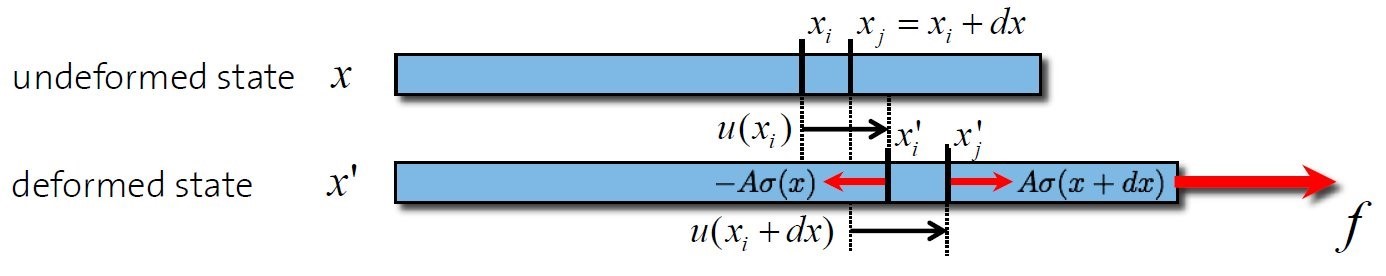
In the un-deformed state Lij = xj − xi and in the deformed state lij = x0j − x0i. Using our previous equation it is possible to derive the strain on the entire segment. As already stated this is of little practical use but by considering the segment as infinitesimally small (namely as dx → 0) then the normal strain at an arbitrary point can be defined as follows:

In a similar fashion to strain, the stress on a segment (force per unit area) can be used to determine the force density at an arbitrary point which is defined as:

This strain displacement relationship enables the force and deformation at any point in a material to be defined and is easily extensible from one to three-dimensions. Consider the 3D deformable body shown in the figure below where the displacement field u(x) describes the deformed body Ω0 in terms of the un-deformed body Ω.
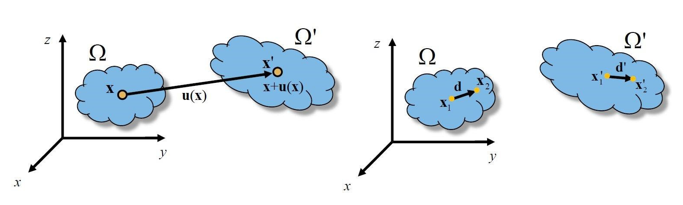
The point x given in material coordinates can be transformed via a function to give the new location described by point x0 in world coordinates where u(x) = x0 − x. To determine the transformation function consider the vector d = x2 − x1 of the un-deformed body (Ω) which is infinitesimal. In the deformed state (Ω0), using the principles previously discussed, this corresponds to the following where F = (I + ∇ u) is known as the deformation gradient or Jacobian and ∇u is a 3x3 matrix with coefficients in the three directional axes.

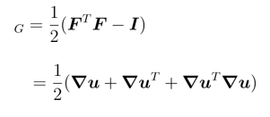
Essentially the deformation gradient can be thought of as describing the change in world coordinates with respect to a change in the material coordinates. As discussed in this fantastic reference book, the Jacobian is invariant to translation (magnitudes are unaffected) but not to rotation and the overall deformation of a given point must be described by measuring the change in length squared in all directions where |d0|2 − |d|2 = d0T d0 − dT d) = dT (F T F − I)d. This leads onto the very important definition of the Green-Lagrange Strain Tensor, a non-linear quadratic entity that is formally defined as:
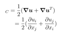
Analysis of this tensor shows that the quadratic term becomes negligible for small displacements and that by removing the non-linear component we arrive at the definition of the linear Cauchy Strain Tensor , where u is the displacement vector, x is the coordinate and the two indices i and j can vary across the three dimensional coordinates x,y,z.
A total of nine strain measures exist as shown in the following equation. 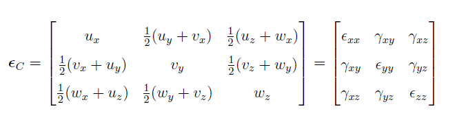 Notationally, E*ij* represents the normal strain previously explored and γij represents the shear strain. It can be thought of as the change in angle of an angle previously at a right angle and represents the total amount of deformation perpendicular to a given axis. Due to the symmetry of this matrix only six independent strain components are needed meaning that the strain can conveniently be rewritten as follows:

It is important to note that the Green strain tensor is rotation-invariant. This can be shown using polar decomposition where any deformation gradient (F 0) can be factored into separate rotation (R) and deformation components (F). Conversely, the Cauchy strain tensor is not rotation-invariant and results in aesthetically displeasing visual artefacts (discussed in a later article).
Stress describes the internal traction forces (T) within a solid - that is the tensile or compressive forces experienced by a continua block - and can be visualised by considering the following figure. E
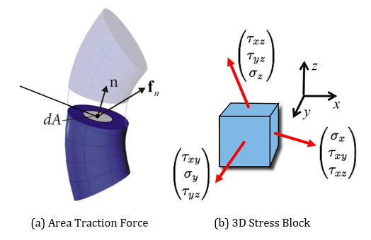
Externally, the body will experience a force per unit area at a given location on the objects surface. This traction is a bound vector that means it can only be fully described by both the force and surface upon which it acts. Internally the process is very similar and by making an arbitrary slice across the object to expose a surface (dA) with a corresponding normal (n) and force (f):
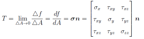
Typically an infinitesimal block within the object, as shown in (b) above, is decomposed into three mutually orthogonal components resulting in the Cauchy Stress Tensor σ . It can be thought of as a set of internal datum planes that are aligned to the x,y,z coordinate system, enabling the stress at any point to be evaluated. The normal stress component ( σ ) is perpendicular to the surface and changes the volume of a material while the shear stress component ( τ ) is tangential to the surface and causes deformation. Similar to the strain tensor, there are only six independent values and the matrix can be simplified to the following tensor. 
CONSTITUTIVE RELATIONS
Stress and strain for a particular material form constitutive equations, a notion that was first suggested by British physicist Robert Hooke and arguably one of the most familiar mathematical expressions where F = −kx. His theory was then generalised by Augustin Cauchy to three dimensional bodies based on the observation that the 6 components of stress are linearly related to the 6 components of strain. This suggests that there are 36 matrix components, true in the general sense but given the conservative nature of most materials and the resulting symmetry of the matrix, this can be reduced to 21 independent components.

The type of material also has a bearing on the complexity of the matrix, as shown in the table above where Triclinic (General Anisotropic) materials have properties dependant on orientation such as the grain on wood. Isotropic materials whose mechanical properties remain the same in all directions are much simpler to consider and the requirements of any computational system are dramatically reduced since only two independent properties are required to define the material - the Young’s Modulus E which embodies the relationship between stress and strain (determining the stiffness of the material in question) and the Poisson Ratio v which is responsible for volume preservation. This can be thought of as materials strained in one direction also experiencing strain in a mutually perpendicular direction despite there being no external loading. Large values of E imply that the material is hard to stretch such as 200GPa for steel or 0.05GPa for more flexible material like rubber.
The Material Property Matrix D can be formed to relate stress to strain:

Further examination of matrix D highlights that, from a computational perspective, only three variables need to be stored giving the following which will greatly reduce storage requirements by eliminating the sparseness of the matrix: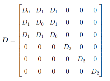
EQUILIBRIUM CONDITIONS
The overall governing equations of an object can be derived by now considering the equilibrium (and boundary) conditions of the body in conjunction with the principles of stress and strain previously discussed. Any object under external loading will reach a state of equilibrium when the net force acting on the body is zero. It is important to note that this balance of forces, or mechanical equilibrium, only occurs when the internal and external forces sum to zero at every point.
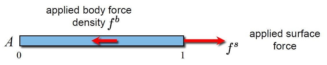
As a simple example, consider the figure above where an axial force fs is applied to a bar in the x-direction only. From early on in our stress/strain equations it is straightforward to see that:
EAux(x) + fb(x) = 0 x ∈]0 , 1[
The governing Partial Differential Equation (PDE) is completely specified by considering the force constraint as fs = EAux(1) and the displacement constraint (or boundary condition) as u(0) = 0. Mathematically this is considered a Boundary Value Problem (BVP) , a framework in which forces, displacements, stresses and strains are connected together before computation for an unknown quantity. The formulation of a BVP, taking into account equilibrium, kinematics and material law, comes in three distinct forms: Strong, Weak and Variational.
- Strong Form
Satisfies each point in the problem domain with strong continuity of the dependant field variables (namely the displacements u,v, and w), with the obvious example being Newton’s second law (F = ma). The PDE discussed above can be considered as being represented in the strong form but, despite offering an exact solution, is difficult to realise practically. Typically the Finite Difference Method (FDM) can be used to discretise the problem so to obtain a finite set of algebraic equations for an approximate solution. This works well for one-dimensional systems (often seen in audio applications) but becomes complicated for non-regular and complex three dimensional domains. From a visual perspective this results in coarse aesthetically displeasing boundary edges, known as the staircase effect, that can suffer from large discretisation errors. This is simply unacceptable for high-quality VFX applications.
- Weak Form
Established using either the integration by parts on a Weighted Residual equation or directly by the Principle of Virtual Work. In a dynamic system the principle of virtual work is replaced by d’Alembert’s Principle which includes an additional inertia term. In both instances only average (integrated) satisfaction of equilibrium is achieved. Such statements were personally quite daunting when first encountered but are simple to conceptualise by referring back to the bar shown in figure 2.4. Consider a test function ¯u that approximates the strong form equation by integrating over the domain:

It then follows that integration by parts of the above equation and the imposition of boundary conditions (fs = EAux(1),¯u(0) = 0) yields the complete governing PDE in weak form, also known as the Virtual Work Equation:

Given that any force F acting through a given distance u performs work such that W = Fu then we can interpret the test function ¯u as a virtual displacement (∂u) . It follows that the virtual displacements across the domain perform no work if and only if the system is in (static) equilibrium. In general, the principle of virtual work states that the stresses, body forces (fb) and tractions (fs) are in equilibrium if the internal work equals the external work for every virtual displacement field. The concept is explained in a general sense here and can be applied to solids or fluids.
• Variational Form
Derived from the Principle of Minimum Potential Energy for static systems or using Hamilton’s Principle for the inclusion of dynamics, which again includes an additional inertia term. It is a form only possible for conservative systems, namely those where work done within the system can be recovered. This form is unattainable when non-conservative forces such as friction are encountered. Owing to the complexity of full variational calculus and that the principle of minimum potential energy is actually derived from the principles of virtual work, the variational form of a BVP will not be explored in this project but interested readers are directed to [15] for further information. Another way of looking at the situation is to consider mechanics, in general, as either Vectorial (based on Newtonian equations) or Analytical (based on energy principles). With this in mind both the weak and variational forms are preferential to the strong form because they use these energy principles to establish fundamental physical insights and functionally express all properties of the model. They are invariant to coordinate transformations since functions are scalar and lead naturally to conservation laws. Both forms are discretised by the Finite Element Method
The following diagram summarises the formulation and subsequent discretisation of the continuum based equations explored thus far:

As with stress and strain, it is relatively straightforward to extend these principles from one to three dimensions by considering the infinitely small block (dx,dy,dz → 0). In the diagram below we assemble the components highlighted in green (which represent the traction forces acting in the x-direction) and the subsequent equation represents the static three-dimensional equilibrium where fx represents an external body force.

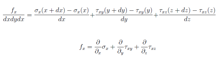
A similar process is used to derive the y and z components to give:
As with the one-dimensional case, the balance of internal and external forces formulates the governing PDE in strong form: ∇σ + fb = 0
It is then possible to formulate the weak form by integrating the strong form, multiplying by the virtual displacement vector ( ∂u) and integrating by parts:
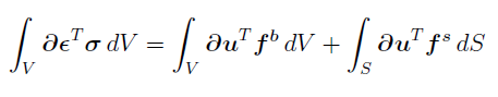
where the internal work performed by stress forces can be seen on the left-hand side of the equation. The external work on the right-hand side is a summation of the forces acting over the volume (V ) of the body and the forces acting on the surface of the body (S). Evidently, ∂u = 0 when on a boundary with a fixed displacement and the virtual strain field is defined as:

REFERENCES
Graham Charles Archer. Object-Oriented Finite Element Analysis. PhD thesis, University of California, Berkeley, 1996.
Bernhard Thomaszewski. Continuum Mechanics and Finite Elements for Deformable Solid Simulation. Computer Graphics Laboratory ETH Zurich, 2011.
Demetri Terzopoulos. Elastically Deformable Models. SIGGRAPH Computer Graphics, 21(4):205–214, 1987.