Generating Noise for applications
Abstract
This article goes into depth around four different types of noise generation algorithms. We cover the implementation as well as performance information for Perlin, Simplex, Wavelet, and Worley noise. This is an analysis of the implementation and the pro’s and cons for each.
Keywords: Noise, Simplex, Wavelet, Value, Worley, Perlin, texturing
Introduction
Noise is a random disturbance in a sample which is not part of an expected result. Think of audio signals on images that you take with your Digital SLR. The noise is the pieces of information that are not desirable such as hiss or speckled spots on low light photos. In these instances this extra information is usually undesirable but in some application this noise makes things more natural and realistic when using random information.
There are many different applications of noise in game development from terrain generation, procedural textures, to artificial intelligence and many more. Noise is surprisingly interesting and is not necessarily just random numbers. Its about how are those numbers distributed how to they relate to previous information. This can be quite a complex topic and in this blog post I will be going through the following types of noise and providing source code and libraries you can leverage to create applications. The types I am going to cover are:
- Value
- Perlin
- Simplex
- Worley
Research Method
The process I am going to take here is focused around implementing and comparing results of each of the noise generation functions. We will compare the following qualitative values:
- Implementation Difficulty
- Resulting graphical noise
The quantitative values we will leverage are:
- Processing time for various image sizes
- Aggregate variance from white
Results
Noise can be a fairly complex topic with a large amount of information on the topic that varies from article to article. We aim to resolve a number of the difficulties with this article as well as provide a complete set of code and framework that can be reused or inspected. Noise functions do not necessarily generate those beautiful pictures you are used to seeing, it’s the layering and adding those layers together which has those various effects.
In order for us to understand these various noise functions we need to compare it to a purely random function. For this we will be leveraging each of the languages random function to generate a number between 0.0f and 1.0f. We will attempt to stick to floating points as much as the language will allows us to. This is in an effort to ensure consistency between the results. Simply put:
  1: function RandomNoise(){
  2:     return random(0.0f,1.0f);
  3: }
1. Random Noise
We take the result of the RandomNoise Function and convert it to an RGB value between 0 and 255. For this article we will stick to shades of grey so the RGB values will all be the same.
1: int r = g = b = randomvalue * 255
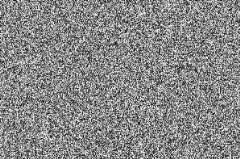
The results of the RandomNoise function look as follows:
Figure 1.0 Noise Pattern
For an image 300px x 200px the average generation time sits in the 1600ms time range in JavaScript. As you can see there is no uniformity to the noise generated. The performance per language is broken down as follows:
| Language | 300x200 | 1024x768 | 1600x900 | 1280x1080 |
| Javascript | 7.6 | 44.8 | 70.6 | 65.6 |
| C# | 3.12358 | 9.37525 | 20.30747 | 20.31865 |
| C++ |
Table 1.0 Random Noise Average Time per resolution
As you can see the performance is purely based on the number of pixels you are trying to generate as well as the language you are using.
Before we go into Perlin Noise there is a bit of understanding of the different types of interpolation that we need to have. Interpolation calculates a projected value between a set of points based on various functions or techniques.
Linear interpolation performs curve fitting using linear polynomials. It takes in 3 inputs Point1, Point2 and t which is a range between 0.0 and 1.0. The function for linear interpolation we will leverage is:
  1: function lerp(v0, v1, t)
  2: {
  3:       return v0+(v1-v0)*t;
  4: }
Cosine interpolation is a form of trigonometric interpolation which will provide us with smoother interpolations than linear. The function we will leverage is:
  1: function cosinerp(v0, v1, t)
  2: {
  3:      ft = t * 3.1415927
  4:      f = (1 - cos(ft)) * .5
  5:      return v0*(1-f) + v1*f
  6: }
Cubic interpolation is a more complex form of interpolation but results in much higher amounts of smoothing between points. Its also one of the simpler options to implement although it does require 4 points and t a range which works similar to the other two versions of interpolation. CatmullRom is a variation of this with weighted multiples applied to the calculation (See source code). The implementation is as follows:
  1: function cuberp(y0, y1,  y2, y3,  mu)
  2: {
  3:      a0,a1,a2,a3,mu2;
  4:      mu2 = mu*mu;
  5:      a0 = y3 - y2 - y0 + y1;
  6:      a1 = y0 - y1 - a0;
  7:      a2 = y2 - y0;
  8:      a3 = y1;
  9:      return(a0*mu*mu2+a1*mu2+a2*mu+a3);
  10: }
Hermite interpolation is similar to Cubic except with the addition of two parameters Tension and Bias. Tension tightens up the curvature of the points and bias twists the curve around specific points. The formula for Hermite interpolation is:
  1: function hermiterp(v0, v1, v2, v3, t, tension, bias){
  2:     var m0,m1,t2,t3;
  3:     var a0, a1, a2, a3;
  4:     t2 = t * t;
  5:     t3 = t2 * t;
  6:     m0  = (v1-v0)*(1+bias)*(1-tension)/2;
  7:     m0 += (v2-v1)*(1-bias)*(1-tension)/2;
  8:     m1  = (v2-v1)*(1+bias)*(1-tension)/2;|
  9:     m1 += (v3-v2)*(1-bias)*(1-tension)/2;
  10:
  11:     a0 =  2*t3 - 3*t2 + 1;
  12:     a1 =    t3 - 2*t2 + t;
  13:     a2 =    t3 -   t2;
  14:     a3 = -2*t3 + 3*t2;
  15:
  16:     return(a0*y1+a1*m0+a2*m1+a3*y2);
  17: }
We also need to understand some terminology before proceeding as I found that without a decent understanding of these terms the following explanations become somewhat difficult to understand first time round. These concepts are focused on how layers are added together and the various properties of the layers.
Octaves: this first term is how many layers of noise are we going to blend together. The more octaves or layers the more detail the noise has
Frequency: this is the number of segments that we are going to put into the space we are using. This is the same as frequency when it comes to sound waves or signal process. The lower the frequency the bigger the features and the higher the frequency the smaller the features.
Amplitude: this is the height of the details. The bigger the amplitude the bigger the height of the features. Generally one will decrease the amplitude for each octave to have a more general smoothing effect.
Persistence: This is the rate at which the amplitude will decrease with each octave that is added. The smaller the persistence the lower the amount of change
With these concepts we can multiply and add various layers of noise together to generate wood like textures, clouds and many other types of procedural textures.
2. Value Noise
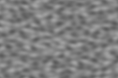
The next one we will look at is Value noise which is one of the simplest. Value noise is a simple algorithm that leverages a grid of random values between 0 and 1 to work out what a pixel should be. Below is a picture of what Value Noise Looks like:
Figure 2.0 Value Noise
The way value noise works is by using a set of points which are randomized and then for each sample between points are interpolated between that set of randomized values. The general flow of this is as follows:
- Generate a set of random values for points
- For the given point calculate the points surrounding
- Get the random value using the surrounding points
- Calculate the difference between the points and use that for your interpolation value
- Interpolate the values
- Return the result
Lets have a look at each of the steps and understand them further. The first stage we generate an array of the appropriate dimension and we assign random values to this. The size of the array can vary quite widely and its worth having a look how the array size affects the out come. For a 2D noise function it will simply be:
  1: for(int x = 0; x < size; x++){
  2:      for(int y = 0; y < size; y++){
  3:           RandomArray[x][y] = Random();
  4:      }
  5: }
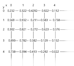
Now we have an array populated with random values this is our noise information that we are going to use to interpolate to have smooth transitions. Lets have a look at how this works. Given a point we map that point to the RandomArray and interpolate the value from the surrounding values points. We also need to know the position of the point given relative to the surrounding points we use this relative information to determine the interpolation value between two points. Now we interpolate and return the value for the noise. Once we populate our grid it should be something similar to this:
Figure 2.1 Populated Random Grid
Say we have a point 2,3 that we want noise for on an image that is 300x200 pixels wide we will pass in the x and y values multiplied by the inverse of the width and height of the area you wish to fill with noise. eg.
tx = 0,0033333 = 1/300
ty = 0,005 = 1/200
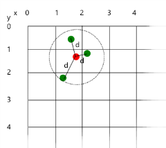
So we pass into the noise function 2.003333 and 3.005 (the red dot on the diagram). We now break down the point passed in into two components, its whole number and the remainder (tx and ty). With the remainder we use a smoothing function to get a new value that is used during interpolation. We then figure out which are the neighbouring points in the generated grid (the green dots on the diagram). We then interpolate the values with each other.
Figure 2.2 The Points used for interpolation to ensure smooth noise.
To view the source code for this please see the source code links in the references section. Below are the performance metrics for the different languages and resolutions.
| Language | 300x200 | 1024x768 | 1600x900 | 1280x1080 |
| Javascript | 8.2 | 94 | 174 | 173 |
| C# | 2.10057 | 58.16069 | 96.27747 | 94.56971 |
| C++ | 1.6 | 4.7 | 3.1 | 0 |
Table 2.0 Value Noise Average Time per resolution
3. Perlin Noise
Perlin Noise is the award winning technique developed by Ken Perlin in 1982 and was leveraged in the motion Picture Tron. It is a gradient noise which is a pseudo random technique. Instead of storing random numbers in the grid as in Value noise and interpolating, Perlin noise stores a gradient vector. To get the values we calculate the dot products of each gradient vector. The dot product is then interpolated to get our result which looks like:
Figure 3.0 Perlin Noise
From the above image you can see Perlin noise is less uniform than Value. There are a number of great articles covering the theory behind Perlin noise which are found in the references section but I will do my best to sum up the jist of what is going on at each step. Looking at Ken Perlin’s improved Perlin noise first step is initializing the array p[]. What is array p? The P array allows us to have a predefined pseudo random allocation of number we can use to generate gradients. We could generate this array using the original method defined by Ken Perlins C code but for performance sake we use a predefined list. This p array is populated to fill 512 items.
Figure 3.1 Populating the P array
Now we have an array that can be used for random numbers we will take our input values and begin processing. It is important to note that the input expected is a floating point (eg 0.0333 or 1.0333). This is why we divide the x and y values by the width and height. This gives us a percentage which is the distance across the width or height. Using this adjusted x and y value as input we then find the cube that surrounds the inputs.
Figure 3.2 Components used for the Perlin Noise calculation
Once we have the required components we now calculate the value that we will be using for the interpolation between the various gradients. This is done using a smoothing function which given a value will return the corresponding value that is on a smoothed curve.
Figure 3.3 Smooth curve values for the Lerp
Using this information we use the values in the p[] array to get hash values that we can leverage to generate the gradients for each point. For example given that our x and y values are (0.0333, 0.0333) for x = 0 and y = 0 the hashes would look as follows:
  1: A = p[0] + 0 = 151
  2: AA = p[A] + 0 = p[151] = 17
  3: …
Using those points we now calculate the various gradients for AA,AB,BA,BB and AA+1, AB+1, BA+1, BB +1.
  1: x = 0.0333
  2: y = 0.0333
  3:  AA = 17
  4:  h = 17 & 15 = 1
  5:  u = 1 < 8 ? 0.0333 : 0.0333 = 0.0333
  6:  v = 1 < 4 ? 1 == 12 || h == 14 ? 0.0333 : 0 = 0
  7:  a = h & 1 == 0 ? u : -u = 0.0333
  8:  b = h & 2 == 0 ? v : -v = 0;
  9:
  10: return a + b = 0.0333
With each of those gradients we now perform a Linear Interpolation between those using the smoothed values and that’s about it.
| Language | 300x200 | 1024x768 | 1600x900 | 1280x1080 |
| Javascript | 22.1 | 259.6 | 447.7 | 440.5 |
| C# | 10.91993 | 178.67824 | 329.77866 | 318.2969 |
| C++ | 4.6 | 40.7 | 70.3 | 78.2 |
Table 3.0 Perlin Noise Average Time per resolution
4. Simplex
Simplex Noise developed by Ken Perlin in 2001 has similar results to Perlin Noise with less computational requirements than Perlin. The idea of Simplex is to divide the N dimensional space into triangles that reduces the number of data points. In Perlin noise we would find the cube that the point we are given in resides and find the points related. Visually the result is not much different from Perlin noise.
Figure 4.0 Simplex Noise
With simplex we are finding the shape that is based on a equilateral triangle and returning fewer points. The major difference Basically it takes the previous grid and skews it and forms triangles for the simplex representation. The gradients for each of the points are then generated and then the rest of the implementation is pretty much the same.
[TODO – Diagram showing the difference between Perlin and Simplex]
The results are good and the performance is much better than Perlin with higher dimensions but it is quite complex to understand
| Language | 300x200 | 1024x768 | 1600x900 | 1280x1080 |
| Javascript | 36.2 | 475.7 | 847.7 | 820.5 |
| C# | 15.75991 | 230.19422 | 418.06524 | 393.17309 |
| C++ | 3 | 107.6 | 192.4 | 182.6 |
Table 4.0 Simplex Noise Average Time per resolution
5. Worley
Worley Noise (Aka Cell Noise) was developed by Steven Worley in 1996 which is very useful in generating stone, water or cell noise textures. The way Worley noise works is that is has a random set of feature points. Given a specific point it calculates the distance of that point to the nearest feature point and uses that for the information. The result is seen below:
Figure 5.0 Worley Noise
What is needed is a set of random points which we compare against. Then we calculate the distance from to the nearest point from the point supplied. Worley’s algorithm has a more efficient implementation of this concept which performs the following steps:
- Calculates which cube a point is in
- Create a random number generator for the cube
- Calculate how many points are inside the cube
- Randomly assign points in the cube
- Find the point closest to the point given
- Check neighboring cubes
- Calculate the distance
Figure 5.1 How the noise value is determined
We can change our results by changing the number of feature points, the way distance is computed and the size of the grid used. If you invert the image you can see the points and the distance information clearly.
| Language | 300x200 | 1024x768 | 1600x900 | 1280x1080 |
| Javascript | 764.8 | 10003.2 | 18879 | 17875.9 |
| C# | 906.9245 | 11532.654 | 21078.3585 | 20539.72 |
| C++ | 290.1 | 3866.4 | 7078.4 | 6615 |
Table 5.0 Worley Noise Average Time per resolution
Conclusion
The various types of noises all have different visual and performance benefits. Below is a visual comparison of each of the different types of noise covered in this article. 
Chart 1.0 Comparison of each of the performance factors across the various languages.By far C++ has the best performance compared to the other languages and C# was typically slower than JavaScript but this can be explained by the direct porting of code instead of using appropriate data structures. The last table summarizes the findings.
Table 6.0 Summarized findings
Source Code:
Sharp Noise : https://sharpnoise.codeplex.com/
References:
Bourke, P (1999) Interpolation Methods, [Online]
Available: https://paulbourke.net/miscellaneous/interpolation/ [7 Feb 2014]
(2012) Noise Part 1, [Online],
Available: https://scratchapixel.com/lessons/3d-advanced-lessons/noise-part-1/ [12 Feb 2014]
(2010) Value_Noise – Explanation of Value Noise, [Online],
Available: https://code.google.com/p/fractalterraingeneration/wiki/Value_Noise [12 Feb 2014]
(2013) Perlin Noise, Wikipedia, [Online],
Available: https://en.wikipedia.org/wiki/Perlin_noise [5 Feb 2014]
Zucker, M (2001) The Perlin noise math FAQ, [Online],
Available: https://webstaff.itn.liu.se/~stegu/TNM022-2005/perlinnoiselinks/perlin-noise-math-faq.html [5 Feb 2014]
Hugo, E (2003) Perlin noise, [Online]
Available: https://freespace.virgin.net/hugo.elias/models/m_perlin.htm [5 Feb 2014]
Perlin, K () Noise and Turbulance, [Online]
Available: https://www.mrl.nyu.edu/~perlin/doc/oscar.html#noise [24 Feb 2014]
Perlin, K () Noise Hardware, [Online]
Available: https://www.csee.umbc.edu/~olano/s2002c36/ch02.pdf [26 Mar 2014]
Perlin, K (2002) Improved Noise Reference Implementation, [Online],
Available: https://mrl.nyu.edu/~perlin/noise/ [7 Feb 2014]
Tulleken, H (2009) How to use Perlin Noise in your games, [Online],
Available: https://devmag.org.za/2009/04/25/perlin-noise/ [7 Feb 2014]
Thomas, K (2011) Perlin Noise in JavaScript, [Online]
Available: https://asserttrue.blogspot.co.uk/2011/12/perlin-noise-in-javascript_31.html [26 Mar 2014]
Explanation of Perlin Noise, [Online]
Available: https://code.google.com/p/fractalterraingeneration/wiki/Perlin_Noise [26 Mar 2014]
Simplex Noise, [Online]
Available: https://en.wikipedia.org/wiki/Simplex_noise [26 Mar 2014]
Gustavson, S (2005) Simplex noise demystified, [Online]
Available: https://webstaff.itn.liu.se/~stegu/simplexnoise/simplexnoise.pdf [26 Mar 2014]
Explanation of Simplex Noise, [Online]
Available: https://code.google.com/p/fractalterraingeneration/wiki/Simplex_Noise [26 Mar 2014]
Worley Noise, [Online]
Available: https://en.wikipedia.org/wiki/Worley_noise [26 Mar 2014]
FreeTheNation (alias) (2013) Cell Noise, [Online]
Available: https://aftbit.com/cell-noise-2/ [26 Mar 2014]
Worley, S, A Cellular Texture Basis Function, [Online]
Available: https://www.rhythmiccanvas.com/research/papers/worley.pdf [26 Mar 2014]
Endre, S (2012) Worley Noise Cellular Texturing, [Online]
Available: https://esimov.com/2012/05/worley-noise-cellular-texturing#.Ux790v_MOM8 [26 Mar 2014]
Nouanesengsy, B CSE 782 Lab 4, [Online]
Available: https://www.cse.ohio-state.edu/~nouanese/782/lab4/ [26 Mar 2014]
Rosen, C (2006) Cell Noise and Processing, [Online]
Available: https://www.carljohanrosen.com/share/CellNoiseAndProcessing.pdf [26 Mar 2014]
Appendix A – Data Results
| 300x200 | 1024x768 | 1600x900 | 1280x1080 | |
| Sample 1 | 51 | 136 | 141 | 73 |
| Sample 2 | 3 | 38 | 65 | 70 |
| Sample 3 | 2 | 34 | 62 | 61 |
| Sample 4 | 2 | 33 | 61 | 59 |
| Sample 5 | 3 | 33 | 62 | 61 |
| Sample 6 | 2 | 37 | 62 | 59 |
| Sample 7 | 4 | 34 | 64 | 69 |
| Sample 8 | 3 | 36 | 63 | 85 |
| Sample 9 | 3 | 35 | 63 | 61 |
| Sample 10 | 3 | 32 | 63 | 58 |
| Average | 7.6 | 44.8 | 70.6 | 65.6 |
Table A.0.1 Javascript Random Noise in milliseconds
| 300x200 | 1024x768 | 1600x900 | 1280x1080 | |
| Sample 1 | 13 | 105 | 157 | 142 |
| Sample 2 | 6 | 87 | 156 | 140 |
| Sample 3 | 7 | 81 | 214 | 237 |
| Sample 4 | 14 | 112 | 236 | 229 |
| Sample 5 | 10 | 115 | 209 | 215 |
| Sample 6 | 6 | 104 | 152 | 150 |
| Sample 7 | 6 | 84 | 147 | 148 |
| Sample 8 | 7 | 88 | 159 | 148 |
| Sample 9 | 7 | 83 | 153 | 168 |
| Sample 10 | 6 | 81 | 157 | 153 |
| Average | 8.2 | 94 | 174 | 173 |
Table A.0.2 Javascript Value Noise in milliseconds
| 300x200 | 1024x768 | 1600x900 | 1280x1080 | |
| Sample 1 | 26 | 266 | 414 | 403 |
| Sample 2 | 28 | 364 | 449 | 423 |
| Sample 3 | 23 | 227 | 432 | 405 |
| Sample 4 | 17 | 246 | 430 | 452 |
| Sample 5 | 16 | 232 | 436 | 468 |
| Sample 6 | 23 | 243 | 442 | 469 |
| Sample 7 | 30 | 258 | 448 | 435 |
| Sample 8 | 17 | 280 | 468 | 448 |
| Sample 9 | 15 | 234 | 482 | 462 |
| Sample 10 | 26 | 246 | 476 | 440 |
| Average | 22.1 | 259.6 | 447.7 | 440.5 |
Table A.0.3 Javascript Perlin Noise in milliseconds
| 300x200 | 1024x768 | 1600x900 | 1280x1080 | |
| Sample 1 | 41 | 498 | 869 | 827 |
| Sample 2 | 35 | 457 | 863 | 874 |
| Sample 3 | 36 | 491 | 893 | 815 |
| Sample 4 | 35 | 474 | 861 | 837 |
| Sample 5 | 36 | 499 | 872 | 849 |
| Sample 6 | 35 | 463 | 822 | 788 |
| Sample 7 | 33 | 440 | 813 | 771 |
| Sample 8 | 33 | 464 | 849 | 862 |
| Sample 9 | 45 | 520 | 823 | 797 |
| Sample 10 | 33 | 451 | 812 | 785 |
| Average | 36.2 | 475.7 | 847.7 | 820.5 |
Table A.0.3 Javascript Simplex Noise in milliseconds
| 300x200 | 1024x768 | 1600x900 | 1280x1080 | |
| Sample 1 | 773 | 9800 | 17970 | 17342 |
| Sample 2 | 752 | 10066 | 18735 | 18308 |
| Sample 3 | 754 | 10432 | 18401 | 18257 |
| Sample 4 | 889 | 11035 | 20495 | 17651 |
| Sample 5 | 761 | 9555 | 18507 | 18100 |
| Sample 6 | 753 | 9934 | 18518 | 18836 |
| Sample 7 | 748 | 10001 | 20718 | 17671 |
| Sample 8 | 715 | 9465 | 17875 | 17159 |
| Sample 9 | 760 | 10047 | 19054 | 17786 |
| Sample 10 | 743 | 9697 | 18517 | 17649 |
| Average | 764.8 | 10003.2 | 18879 | 17875.9 |
Table A.0.4 Javascript Worley Noise in milliseconds
| 300x200 | 1024x768 | 1600x900 | 1280x1080 | |
| Sample 1 | 15,6219 | 15,6259 | 15,6243 | 31,2802 |
| Sample 2 | 0 | 0 | 31,2503 | 15,6251 |
| Sample 3 | 0 | 15,6264 | 15,6251 | 15,6267 |
| Sample 4 | 0 | 15,6239 | 15,6247 | 15,626 |
| Sample 5 | 15,6239 | 0 | 15,6259 | 31,2503 |
| Sample 6 | 0 | 0 | 31,251 | 15,6264 |
| Sample 7 | 0 | 15,6243 | 15,5984 | 15,6518 |
| Sample 8 | 0 | 15,6264 | 15,6259 | 15,6243 |
| Sample 9 | 0 | 15,6256 | 15,598 | 31,2781 |
| Sample 10 | 0 | 0 | 31,2511 | 15,5976 |
| Average | 3,12458 | 9,37525 | 20,30747 | 20,31865 |
C# Random Noise
| 300x200 | 1024x768 | 1600x900 | 1280x1080 | |
| Sample 1 | 0 | 62,4993 | 93,7827 | 93,7233 |
| Sample 2 | 0 | 62,5292 | 93,7515 | 93,7524 |
| Sample 3 | 0 | 62,5009 | 93,754 | 93,7216 |
| Sample 4 | 0 | 62,5309 | 93,7228 | 93,7819 |
| Sample 5 | 0 | 62,5017 | 93,7516 | 98,6821 |
| Sample 6 | 4,0003 | 54,0036 | 99,9782 | 94,0085 |
| Sample 7 | 4,0003 | 55,0332 | 99,006 | 94,0094 |
| Sample 8 | 3,9999 | 53,0043 | 101,0083 | 95,0069 |
| Sample 9 | 5,0008 | 53,0039 | 97,008 | 95,0032 |
| Sample 10 | 4,0044 | 53,9999 | 97,0116 | 94,0078 |
| Average | 2,10057 | 58,16069 | 96,27747 | 94,56971 |
C# Value Noise
| 300x200 | 1024x768 | 1600x900 | 1280x1080 | |
| Sample 1 | 3,0671 | 187,5339 | 328,1042 | 312,5086 |
| Sample 2 | 0 | 187,5314 | 312,4794 | 328,1621 |
| Sample 3 | 0 | 187,4756 | 328,1596 | 296,8797 |
| Sample 4 | 15,6276 | 187,5044 | 328,1329 | 296,8814 |
| Sample 5 | 15,6259 | 171,8792 | 328,105 | 312,5053 |
| Sample 6 | 15,6256 | 171,9055 | 328,1324 | 323,6092 |
| Sample 7 | 14,001 | 179,0144 | 329,0262 | 328,0242 |
| Sample 8 | 14,0022 | 164,5815 | 328,1325 | 312,5077 |
| Sample 9 | 15,6252 | 187,4768 | 312,5345 | 312,5077 |
| Sample 10 | 15,6247 | 171,8797 | 374,9799 | 359,3831 |
| Average | 10,91993 | 179,67824 | 329,77866 | 318,2969 |
C# Perlin Noise
| 300x200 | 1024x768 | 1600x900 | 1280x1080 | |
| Sample 1 | 15,6272 | 265,6312 | 468,759 | 390,6362 |
| Sample 2 | 15,6235 | 218,785 | 399,3286 | 390,6338 |
| Sample 3 | 15,6255 | 218,755 | 421,8578 | 400,3869 |
| Sample 4 | 16,9734 | 223,7623 | 406,2314 | 453,1643 |
| Sample 5 | 15,6255 | 281,228 | 437,5071 | 390,6379 |
| Sample 6 | 15,6226 | 218,7575 | 406,2581 | 375,0374 |
| Sample 7 | 15,6255 | 218,7275 | 421,9124 | 374,9803 |
| Sample 8 | 15,6252 | 218,7841 | 406,2589 | 375,0087 |
| Sample 9 | 15,6251 | 218,7562 | 406,2528 | 390,6395 |
| Sample 10 | 15,6256 | 218,7554 | 406,2593 | 390,6059 |
| Average | 15,75991 | 230,19422 | 418,06254 | 393,17309 |
C# Simplex Noise
| 300x200 | 1024x768 | 1600x900 | 1280x1080 | |
| Sample 1 | 875,0507 | 11721,8289 | 21159,6973 | 20796,8689< |
| Sample 2 | 881,7512 | 11395,9728 | 21601,9663 | 21163,0641< |
| Sample 3 | 937,5188 | 11781,6182 | 21021,7052 | 20026,9773< |
| Sample 4 | 875,0204 | 11425,826 | 20934,028 | 20934,7304 |
| Sample 5 | 968,7906 | 11538,2469 | 20978,2407 | 20503,3906< |
| Sample 6 | 875,015 | 11437,8304 | 21050,5453 | 20282,7218 |
| Sample 7 | 859,3624 | 11500,553 | 21201,9371 | 20710,8594 |
| Sample 8 | 1046,8467 | 11692,1106 | 21034,7107 | 20608,7085 |
| Sample 9 | 874,9585 | 11458,6809 | 20889,1269 | 19987,1211< |
| Sample 10 | 874,931 | 11373,8703 | 20911,6274 | 20382,7533< |
| Average | 906,92453 | 11532,6538 | 21078,35849 | 20539,7195 |
C# Worley Noise
| 300x200 | 1024x768 | 1600x900 | 1280x1080 | |
| Sample 1 | 0 | 0 | 0 | 0 |
| Sample 2 | 0 | 0 | 0 | 0 |
| Sample 3 | 0 | 0 | 0 | 0 |
| Sample 4 | 0 | 0 | 0 | 0 |
| Sample 5 | 16 | 0 | 0 | 0 |
| Sample 6 | 0 | 15 | 0 | 0 |
| Sample 7 | 0 | 16 | 0 | 0 |
| Sample 8 | 0 | 16 | 0 | 0 |
| Sample 9 | 0 | 0 | 15 | 0 |
| Sample 10 | 0 | 0 | 16 | 0 |
| Average | 1.6 | 4.7 | 3.1 | 0 |
C++ Random Noise
| 300x200 | 1024x768 | 1600x900 | 1280x1080 | |
| Sample 1 | 0 | 47 | 78 | 79 |
| Sample 2 | 15 | 31 | 79 | 78 |
| Sample 3 | 15 | 32 | 78 | 78 |
| Sample 4 | 0 | 32 | 78 | 78 |
| Sample 5 | 0 | 46 | 63 | 78 |
| Sample 6 | 0 | 47 | 62 | 78 |
| Sample 7 | 0 | 47 | 62 | 78 |
| Sample 8 | 0 | 47 | 62 | 78 |
| Sample 9 | 16 | 47 | 62 | 79 |
| Sample 10 | 0 | 31 | 79 | 78 |
| Average | 4.6 | 40.7 | 70.3 | 78.2 |
C++ Value Noise
| 300x200 | 1024x768 | 1600x900 | 1280x1080 | |
| Sample 1 | 16 | 109 | 187 | 188 |
| Sample 2 | 16 | 109 | 187 | 188 |
| Sample 3 | 16 | 109 | 187 | 172 |
| Sample 4 | 16 | 93 | 203 | 170 |
| Sample 5 | 16 | 109 | 188 | 187 |
| Sample 6 | 0 | 109 | 188 | 187 |
| Sample 7 | 0 | 109 | 188 | 187 |
| Sample 8 | 0 | 109 | 188 | 187 |
| Sample 9 | 16 | 93 | 194 | 188 |
| Sample 10 | 16 | 94 | 203 | 187 |
| Average | 11.2 | 104.3 | 191.3 | 184.1 |
C++ Perlin Noise
| 300x200 | 1024x768 | 1600x900 | 1280x1080 | |
| Sample 1 | 15 | 110 | 187 | 172 |
| Sample 2 | 15 | 94 | 203 | 172 |
| Sample 3 | 0 | 109 | 188 | 187 |
| Sample 4 | 0 | 109 | 188 | 187 |
| Sample 5 | 0 | 109 | 188 | 187 |
| Sample 6 | 0 | 109 | 188 | 187 |
| Sample 7 | 0 | 109 | 188 | 187 |
| Sample 8 | 0 | 109 | 203 | 172 |
| Sample 9 | 0 | 109 | 188 | 187 |
| Sample 10 | 0 | 109 | 203 | 188 |
| Average | 3 | 107.6 | 192.4 | 182.6 |
C++ Simplex Noise
| 300x200 | 1024x768 | 1600x900 | 1280x1080 | |
| Sample 1 | 281 | 3776 | 6672 | 6992 |
| Sample 2 | 312 | 3719 | 7014 | 6674 |
| Sample 3 | 281 | 4266 | 7453 | 6719 |
| Sample 4 | 281 | 4156 | 7954 | 6922 |
| Sample 5 | 281 | 3859 | 7385 | 6484 |
| Sample 6 | 297 | 4063 | 6797 | 6487 |
| Sample 7 | 313 | 3894 | 6992 | 6435 |
| Sample 8 | 281 | 3619 | 6915 | 6365 |
| Sample 9 | 277 | 3705 | 6728 | 6634 |
| Sample 10 | 297 | 3607 | 6874 | 6438 |
| Average | 290.1 | 3866.4 | 7078.4 | 6615 |
C++ Worley Noise
