Pixel-Level Land Cover Classification Using the Geo AI Data Science Virtual Machine and Batch AI
This post was authored by Mary Wahl, Kolya Malkin, Siyu Yang, Patrick Flickinger, Wee Hyong Tok, Lucas Joppa, and Nebojsa Jojic, representing the Microsoft Research and AI for Earth teams.
Last week Microsoft launched the Geo AI Data Science Virtual Machine (DSVM), an Azure VM type specially tailored to data scientists and analysts that manage geospatial data. To support the Geo AI DSVM launch, we are sharing sample code and methods for our joint land cover mapping project with the Chesapeake Conservancy and ESRI. We have used Microsoft’s Cognitive Toolkit (CNTK) to train a deep neural network-based semantic segmentation model that assigns land cover labels from aerial imagery. By reducing cost and speeding up land cover map construction, such models will enable finer-resolution timecourses to track processes like deforestation and urbanization. This blog post describes the motivation behind our work and the approach we’ve taken to land cover mapping. If you prefer to get started right away, please head straight to our GitHub repository to find our instructions and materials.
Motivation for the Land Cover Mapping Use Case
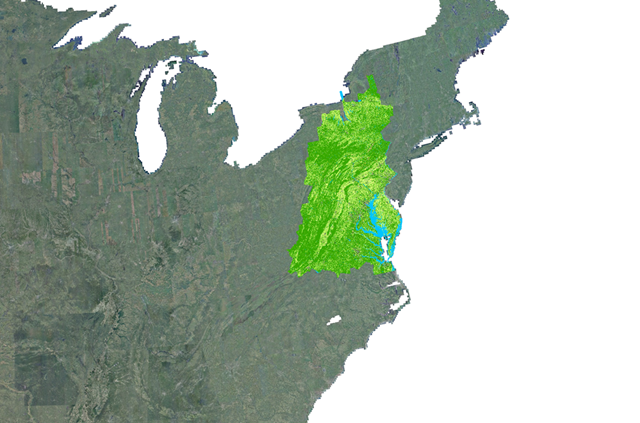
The Chesapeake Conservancy is a non-profit organization charged with monitoring natural resources in the Chesapeake Bay watershed, a >165,000 square kilometer region in the eastern U.S. extending from New York through Virginia. For a year and a half, the Chesapeake Conservancy spearheaded work with the Chesapeake Bay Program Partnership, WorldView Solutions, and University of Vermont Spatial Analysis Laboratory to meticulously assign each square meter in this region a land cover label such as water, grass/herbaceous, tree/forest, or barren/impervious surface. The resulting high-quality, high-resolution land cover map reflects 2013/2014 ground conditions and is a valuable resource already used by environmental scientists and conservation efforts throughout the region. If similar maps could be generated at frequent timepoints, the data would allow researchers to quantify trends such as deforestation, urbanization, and the impacts of climate change.

Unfortunately, cost and time required for land cover map construction currently limit how frequently such maps can be produced. The Chesapeake Conservancy used several input data sources that had to be collected at the municipality, county, or state level, including LiDAR (to estimate height), multi-seasonal aerial imagery, and smaller-scale land use maps. In addition to the burden of assembling and curating these data sources, the Chesapeake Conservancy manually corrected errors because the rule-based classification workflow used for first-pass predictions of land cover labels was insufficiently accurate.
Our Land Cover Mapping Model
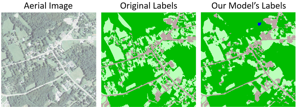
In collaboration with the Chesapeake Conservancy and ESRI, we at Microsoft helped train a deep neural network model to predict land cover from a single high-resolution aerial imagery data source collected nationwide at frequent intervals. We produced a neural network similar in architecture to Ronnenberger et al.’s U-net (2015), a commonly-used semantic segmentation model type. Our trained model’s predictions show excellent agreement with Chesapeake Conservancy’s land cover map. Some discrepancies reflect outdated or erroneous information in the original land cover map, including the small pond in the example below:

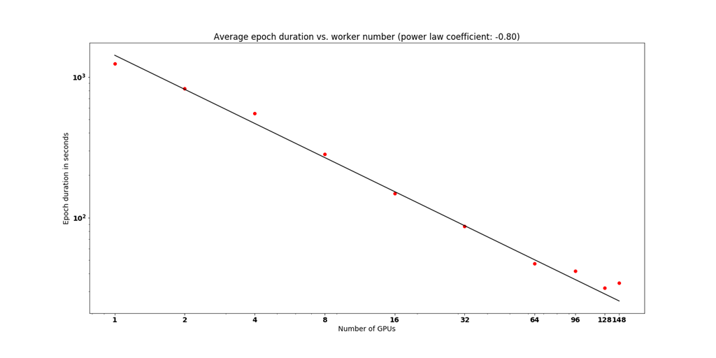
After prototyping the training method on a single-GPU Azure Deep Learning Virtual Machine with a subset of available data, we scaled up training to a 148-GPU cluster using Azure Batch AI. This transition allowed us to reduce the average duration of each training epoch forty-fold, and further reduced runtime by allowing the complete ~1 TB training dataset to be stored in memory rather than repeatedly accessed from disk.

We also addressed issues common with geospatial datasets such as making efficient use of very large, paired training image files (typical size: ~1 GB), label imbalance, and accommodating partial missingness of labels. Microsoft’s Cognitive Toolkit (CNTK) provided the flexibility needed to provide a custom data import method and loss function, while also simplifying the transition from single-process to distributed training.
Training and Applying the Model
Our pixel-level land classification tutorial contains both Jupyter notebooks for training the model on a single Geo AI DSVM, as well as instructions for training the model at scale using Batch AI. (You’re also welcome to adapt these files and methods for other types of computers, but you may find that you need to install some dependencies and ensure you have adequate hardware.) If you deploy a Geo AI DSVM, you’ll find copies of the Jupyter notebooks for this tutorial pre-installed in the “notebooks” folder under the user account’s home directory. Geo AI DSVMs can be created with 1, 2, or 4 NVIDIA K80 GPUs using VM sizes named NC6, NC12, and NC24, respectively: if you opt for multiple GPUs, you’ll also be able to test out the speed-up afforded by data-parallel distributed training.
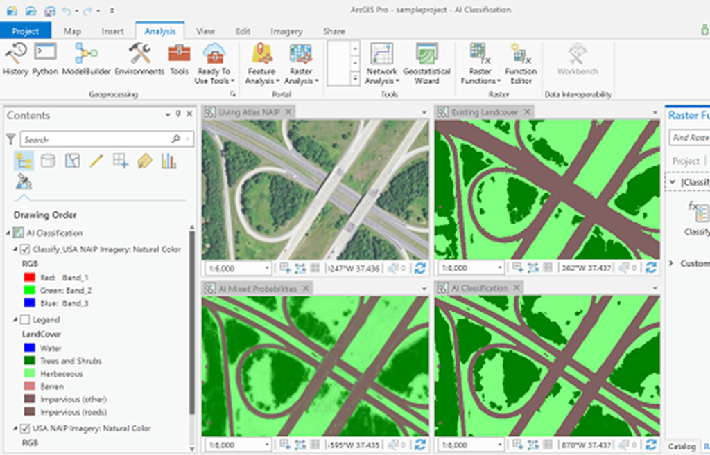
Our Geo AI DSVM notebooks culminate by surfacing our trained model inside ESRI’s ArcGIS Pro, which comes pre-installed on the Geo AI DSVM. For researchers and analysts who work frequently with geospatial data, the ArcGIS software suite will be a familiar tool: it’s often used to create maps from raster or vector data, and to perform analyses that make use of spatial information. ArcGIS Pro is also a useful visualization tool: information can be computed and displayed in real-time while navigating through maps. ESRI’s Hua Wei has developed a custom raster function that can be used to call our land cover classification model in real-time and display the results alongside the original imagery and true labels: the code and sample ArcGIS project he developed, along with instructions on how to use them, are provided in our tutorial. While “ground-truth” labels are only available in the Chesapeake Bay watershed, you’ll be able to see the model’s predictions for regions throughout the continental U.S. in real-time.

Next Steps
We hope you enjoy our pixel-level land classification tutorial! We are very grateful to the Chesapeake Conservancy and ESRI for their help throughout this project and for allowing their data, trained models, and code to be shared here.
Please visit the following pages to learn more:
- Visit our GitHub repository for instructions on starting the tutorials.
- Read more about AI for Earth.
- Read the Batch AI product page, recipes, and documentation.
- Read more about the Geo AI DSVM.
See our related example on embarrassingly-parallel classification of aerial images.
Mary, Kolya, Siyu, Patrick, Wee Hyong, Lucas & Nebojsa