From Stumps to Trees to Forests
This blog post is authored by Chris Burges , Principal Research Manager at Microsoft Research, Redmond.
In my last post we looked at how machine learning (ML) provides us with adaptive learning systems that can solve a wide variety of industrial strength problems, using Web search as a case study. In this post I will describe how a particularly popular class of learning algorithms called boosted decision trees (BDTs) works. I will keep the discussion at the ideas level, rather than give mathematical details, and focus here on the background you need to understand BDTs. I mentioned last time that BDTs are very flexible and can be used to solve problems in ranking (e.g. how should web search results be ordered?), classification (e.g., is an email spam or not?) and regression (e.g., how can you predict what price your house will sell for?). Of these, the easiest to describe is the binary classification task (that is, the classification task where one of two labels is attached to each item), so let’s begin with that.
A BDT model is a collection (aka ensemble) of binary decision trees (that is, decision trees in which each internal node has two children), each of which attempts to solve part of the problem. To understand how single decision trees work let’s consider the simplest possible decision tree, known as a decision stump, which is just a tree with two leaf nodes. To make things concrete, let’s consider the classification task of predicting someone’s gender based only on other information, and to start with, let’s assume that we only know their height. A decision stump in this case looks like this:
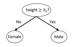
Thus, the decision stump asserts that if a person’s height h is less than a threshold height ht, then that person is female, else male. The parameter ht is found using a “training set” of labeled data by determining that ht such that, if a leaf node asserts male or female based on the majority vote of the labels of the training samples that land there, the overall error rate on that training set is minimized. It is always possible to pick such a threshold: the corresponding error rate is known as the Bayes error. Let’s suppose we have such a training set and that doing this yields ht = 1.4 meters.
Now of course there are tall women and short men, and so we expect the Bayes error to be nonzero. How might we build a system that has a lower error rate? Well, suppose we also have access to additional data, such as the person’s weight w. Our training set now looks like a long list of tuples of type (height, weight, gender). The input data types (height and weight) are called features. The training data will also have labels (gender) but of course the test data won’t, and our task is to predict well on previously unseen data. We haven’t gone far yet, but we’ve already run into three classic machine learning issues: generalization, feature design, and greedy learning. Machine learning usually pins its hopes on the assumption that the unseen (test) data is distributed similarly to the training set, so let’s adopt that assumption here (otherwise we will have no reason to believe that our model will generalize, that is, perform well on test data). Regarding feature design, we could just use h and w as features, but we know that they will be strongly correlated: perhaps a measure of density such as w/h would be a better predictor (i.e. result in splits with lower Bayes error). If it so happened that w/h is an excellent predictor, the tree that approximates this using only w and h would require many more splits (and be much deeper) than one that can split directly on w/h. So perhaps we’d settle on h, w and w/h as our feature set. As you can see, feature design is tricky, but a good rule of thumb is to find as many features as possible that are largely uncorrelated, yet still informative, to pick the splits from.
Notice that our features have different dimensions – in the metric system, h is measured in meters, w in kilograms, and w/h is measured in kilograms per meter. Other machine learning models such as neural networks will happily do arithmetic on these features, which works fine as long as the data is not scaled; but it does seem odd to be adding and comparing quantities that have different dimensions (what does it mean to add a meter to a kilogram?). Decision trees do not have this problem because all comparisons are done on individual features: for example it seems more natural to declare that if a person’s linear density is larger than 40 kilos per meter, and their height is greater than 1.8 meters, then that person is likely male. If after training, some law was passed requiring that all new data be represented in Imperial rather than in Metric units, for any machine learning system we can simply scale the new data back to what the system was trained on; but for trees we have an alternative, namely to rescale the comparison in each node, in this case from Metric to Imperial units. (Not handling such rescaling problems correctly can cause big headaches, such as the loss of one’s favorite Mars orbiter.)
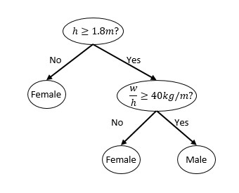
Regarding greediness, when growing the tree, choosing all of its splits simultaneously to give the overall optimal set of splits is a combinatorically hard problem, so instead we simply scan each leaf node and choose the node and split that results in lowest overall Bayes error. This often works well but there are cases (we’ll look at one below) for which it fails miserably. So, after two splits our decision tree might look like this, where we’ve put in the concrete values found by minimizing the error on a training set:
Now let’s turn to that miserable failure. Suppose the task is to determine the parity of a 100-bit bit vector (that is, whether the total number of bits is even or odd, not whether the vector represents an even or odd number!), and that for training data we’re given access to an unlimited number of labeled vectors. Any choice of bit position to split on in the first node will give the worst possible Bayes error of ½ (up to small statistical fluctuations, whose size depends on the size of the training set we wind up using). The only binary tree that can fully solve this will have to have depth 100, with 1,267,650,600,228,229,401,496,703,205,376 leaf nodes. Even if this were practical to do, the tree would have to be constructed by hand (i.e. not using the greedy split algorithm) because even at the penultimate layer of the tree (one layer above the leaf nodes), any split still gives Bayes error of ½. Clearly this algorithm won’t work for this task, which can be solved in nanoseconds by performing ninety nine XOR operations in sequence. The problem is that trying to split the task up at the individual bit level won’t work. As soon as we are allowed to consider more than one bit at a time (just two, in the case of XOR) we can solve the problem very efficiently. This might look like a minor concern, but it does illustrate that greedily trained trees aren’t likely to work as well on tasks for which the label depends only on combinations of many features.
Let’s look now at binary trees for regression. Binary classification may be viewed as a special case of regression in which the targets take only two values. The case in which the targets take on more than two values, but still a finite number of values, can be thought of as multiclass classification (for example: identify the species of animal shown in a photo). The case in which the targets take on a continuum of values, so that a feature vector x maps to a number f(x), where f is unknown, is the general regression task. In this case the training data consists of a set of feature vectors xi (for example, for the house price prediction problem, the number of bedrooms, the quality of the schools, etc.) each with f( xi ) (the selling price of the house) provided, and the task is to model f so that we can predict f(x) for some previously unseen vector x. How would a tree work in this more general case? Ideally we would like a given leaf to contain training samples that all have the same f value (say, f0), since then prediction is easy – we predict that any sample that falls in that leaf has f value equal to f0. However there will almost always be a range of f values in a given leaf, so instead we try to build the tree so that each leaf has the smallest such range possible (i.e. the variances of the f values in its leaves are minimized) and we simply use the mean value of the f values in a given leaf as our prediction for that leaf. We have just encountered a fourth classic machine learning issue: choice of a cost function. For simplicity we will stick with the variance as our cost function, but several others can also be used.
So now we know how to train and test with regression trees: during training, loop through the current leaves and split on that leaf, and feature, that gives the biggest reduction in variance of the f’ s. During test phase, see which leaf your sample falls to and declare your predicted value as the mean of the f’s of the training samples that fell there. However this raises the question: does it make sense to split if the number of training samples in the leaf is small? For example, if it’s two, then any split will reduce the variance of that leaf to zero. Thus looms our fifth major issue in machine learning: regularization, or the avoidance of overfitting. Overfitting occurs when we tune to the training data so well that accuracy on test data begins to drop; we are learning particular vagaries of our particular training set, which don’t transfer to general datasets (they don’t “generalize”). One common method to regularize trees is indeed to stop splitting when the number of training samples in a leaf falls below a fixed, pre-chosen threshold value (that might itself be chosen by trying out different values and seeing which does best on a held-out set of labeled data).
The regression tree is a function (that maps each data point to a real number). It is a good rule to use only the simplest function one can to fit the training data, to avoid overfitting. Now, for any positive integers n and k, a tree with nk leaves has nk -1 parameters (one for the split threshold at each internal node). Suppose instead that we combine k trees, each with n leaves, using k-1 weights to linearly combine the outputs of the k-1 trees with the first. This model can also represent exactly nk different values, but it has only nk-1 parameters – exponentially fewer than the single tree. This fits our “Occam’s Razor” intuition nicely, and indeed we find that using such “forests”, or ensembles of trees, instead of a single tree, often achieves higher test accuracy for a given a training set. The kinds of functions the two models implement are also different. When the input data has only two features (is two dimensional), each leaf in a tree represents an axis-parallel rectangular region in the plane (where the rectangles may be open, that is, missing some sides). For data with more than two dimension the regions are hyper-rectangles (which are just the high dimensional analog of rectangles). An ensemble of trees, however, is taking a linear combination of the values associated with each rectangle in a set of rectangles that all overlap at the point in question. But, do we lose anything by using ensembles? Yes: interpretability of the model. For a single tree we can follow the decisions made to get to a given leaf and try to understand why they were sensible decisions for the data in that leaf. But except for small trees it’s hard to make sense of the model in this way, and for ensembles, it’s even harder.
So, finally, what is boosting? The idea is to build an ensemble of trees, and to use each new tree to try to correct the errors made by the ensemble built so far. AdaBoost was the first boosting algorithm to become widely adopted for practical (classification) problems. Boosting is a powerful idea that is principled (meaning that one can make mathematical statements about the theory, for example showing that the model can learn even if, for the classification task, each subsequent tree does only slight better than random guessing on the task) and very general (one can solve a wide range of machine learning problems, each with its own cost function, with it). A particularly general and powerful way to view boosting is as gradient descent in function space, which makes it clear how to adapt boosting to new tasks. In that view, adding a new tree is like taking a step downhill in the space in which the functions live, to find the best overall function for the task at hand.
To go much further would require that I break my promise of keeping the ideas high level and non-mathematical, so I will stop here – but the math is really not hard, and if you’re interested, follow the links above and the references therein to find out more. If you’d like to try BDTs for yourself, you can use the Scalable Boosted Decision Trees module in AzureML to play around and build something cool.
Chris Burges
Learn about my research.