レシピ: Azure AI サービス - 多変量異常検出

[アーティクル]
02/05/2024

このレシピでは、Apache Spark で SynapseML と Azure AI サービスを使用して多変量異常検出を実行する方法を示します。多変量異常検出では、さまざまな変数間のすべての内部的な関連性と依存関係を考慮に入れながら、多くの変数または時系列間の異常を検出できます。このシナリオでは、SynapseML を使用して、Azure AI サービスを使用した多変量異常検出用のモデルをトレーニングし、その後、そのモデルを使用して、3 つの IoT センサーからの合成測定値を含むデータセット内の多変量異常を推論します。

重要

2023 年 9 月 20 日以降は、新しい Anomaly Detector リソースを作成できなくなります。 Anomaly Detector サービスは、2026 年 10 月 1 日に廃止されます。

Azure AI Anomaly Detector の詳細については、こちらのドキュメントページを参照してください。

前提条件

Azure サブスクリプション - 無料アカウントを作成します
ノートブックをレイクハウスにアタッチします。左側の [追加] を選択して、既存のレイクハウスを追加するか、レイクハウスを作成します。

セットアップ

手順に従って、Azure portal を使用して Anomaly Detector リソースを作成します。または Azure CLI を使用してこのリソースを作成することもできます。

Anomaly Detector を設定すると、さまざまな形式のデータを処理する方法を見ることができます。 Azure AI 内のサービスのカタログには、Vision、Speech、Language、Web Search、Decision、Translation、Document Intelligence という複数のオプションが用意されています。

Anomaly Detector リソースを作成する

Azure portal のリソースグループで [作成] を選択し、"Anomaly Detector" と入力します。 Anomaly Detector リソースを選択します。
リソースに名前を付けます。また、リソースグループの他の部分と同じリージョンを使用するのが理想的です。残りの部分には既定のオプションを使用し、[確認 + 作成] を選択して [作成] を選択します。
Anomaly Detector リソースが作成されたら、それを開いて、左側ナビゲーションにある [Keys and Endpoints] パネルを選択します。 Anomaly Detector リソースのキーを ANOMALY_API_KEY 環境変数にコピーするか、anomalyKey 変数に保存します。

ストレージアカウントリソースを作成する

中間データを保存するには、Azure Blob Storage アカウントを作成する必要があります。そのストレージアカウント内に、中間データを保存するためのコンテナーを作成します。コンテナー名をメモし、接続文字列をそのコンテナーにコピーします。これは、後で containerName 変数と BLOB_CONNECTION_STRING 環境変数を設定するために必要になります。

サービスキーの入力

まず、サービスキーの環境変数を設定しましょう。次のセルでは、Azure Key Vault に保存されている値に基づいて、ANOMALY_API_KEY および BLOB_CONNECTION_STRING 環境変数を設定します。このチュートリアルを独自の環境で実行している場合は、続行する前に、これらの環境変数を設定してください。

import os
from pyspark.sql import SparkSession
from synapse.ml.core.platform import find_secret

# Bootstrap Spark Session
spark = SparkSession.builder.getOrCreate()

次に、ANOMALY_API_KEY および BLOB_CONNECTION_STRING 環境変数を読み取り、containerName および location 変数を設定しましょう。

# An Anomaly Dectector subscription key
anomalyKey = find_secret("anomaly-api-key") # use your own anomaly api key
# Your storage account name
storageName = "anomalydetectiontest" # use your own storage account name
# A connection string to your blob storage account
storageKey = find_secret("madtest-storage-key") # use your own storage key
# A place to save intermediate MVAD results
intermediateSaveDir = (
    "wasbs://madtest@anomalydetectiontest.blob.core.windows.net/intermediateData"
)
# The location of the anomaly detector resource that you created
location = "westus2"

まず、異常検出機能で中間結果を保存できるように、ストレージアカウントに接続します。

spark.sparkContext._jsc.hadoopConfiguration().set(
    f"fs.azure.account.key.{storageName}.blob.core.windows.net", storageKey
)

必要なすべてのモジュールをインポートしてみましょう。

import numpy as np
import pandas as pd

import pyspark
from pyspark.sql.functions import col
from pyspark.sql.functions import lit
from pyspark.sql.types import DoubleType
import matplotlib.pyplot as plt

import synapse.ml
from synapse.ml.cognitive import *

次に、サンプルデータを Spark データフレームに読み込みましょう。

df = (
    spark.read.format("csv")
    .option("header", "true")
    .load("wasbs://publicwasb@mmlspark.blob.core.windows.net/MVAD/sample.csv")
)

df = (
    df.withColumn("sensor_1", col("sensor_1").cast(DoubleType()))
    .withColumn("sensor_2", col("sensor_2").cast(DoubleType()))
    .withColumn("sensor_3", col("sensor_3").cast(DoubleType()))
)

# Let's inspect the dataframe:
df.show(5)

これで、モデルのトレーニングに使用される estimator オブジェクトを作成できるようになりました。トレーニングデータの開始および終了時刻を指定します。また、使用する入力列と、タイムスタンプを含む列の名前も指定します。最後に、異常検出スライディングウィンドウで使用するデータポイントの数を指定し、接続文字列を Azure Blob Storage アカウントに設定します。

trainingStartTime = "2020-06-01T12:00:00Z"
trainingEndTime = "2020-07-02T17:55:00Z"
timestampColumn = "timestamp"
inputColumns = ["sensor_1", "sensor_2", "sensor_3"]

estimator = (
    FitMultivariateAnomaly()
    .setSubscriptionKey(anomalyKey)
    .setLocation(location)
    .setStartTime(trainingStartTime)
    .setEndTime(trainingEndTime)
    .setIntermediateSaveDir(intermediateSaveDir)
    .setTimestampCol(timestampColumn)
    .setInputCols(inputColumns)
    .setSlidingWindow(200)
)

estimator が作成されたので、これをデータに当てはめてみましょう。

model = estimator.fit(df)
```parameter

Once the training is done, we can now use the model for inference. The code in the next cell specifies the start and end times for the data we would like to detect the anomalies in.

```python
inferenceStartTime = "2020-07-02T18:00:00Z"
inferenceEndTime = "2020-07-06T05:15:00Z"

result = (
    model.setStartTime(inferenceStartTime)
    .setEndTime(inferenceEndTime)
    .setOutputCol("results")
    .setErrorCol("errors")
    .setInputCols(inputColumns)
    .setTimestampCol(timestampColumn)
    .transform(df)
)

result.show(5)

前のセルで .show(5) を呼び出すと、データフレームの最初の 5 行が表示されました。推論ウィンドウ内になかったため、結果はすべて null でした。

推論されたデータの結果のみを表示するために、必要な列を選択しましょう。その後、データフレーム内の行を昇順で並べ替え、結果をフィルター処理することで、推論ウィンドウの範囲内にある行のみを表示できます。この場合 inferenceEndTime は、データフレームの最後の行と同じであるため、無視できます。

最後に、結果をより適切にプロットできるように、Spark データフレームを Pandas データフレームに変換します。

rdf = (
    result.select(
        "timestamp",
        *inputColumns,
        "results.contributors",
        "results.isAnomaly",
        "results.severity"
    )
    .orderBy("timestamp", ascending=True)
    .filter(col("timestamp") >= lit(inferenceStartTime))
    .toPandas()
)

rdf

次に、検出された異常に対応する各センサーからの寄与度スコアを保存する、contributors 列を形式化します。次のセルは、このデータの書式を設定し、各センサーの寄与スコアを独自の列に分割します。

def parse(x):
    if type(x) is list:
        return dict([item[::-1] for item in x])
    else:
        return {"series_0": 0, "series_1": 0, "series_2": 0}

rdf["contributors"] = rdf["contributors"].apply(parse)
rdf = pd.concat(
    [rdf.drop(["contributors"], axis=1), pd.json_normalize(rdf["contributors"])], axis=1
)
rdf

すばらしい。これで、センサー 1、2、および 3 の寄与スコアがそれぞれ series_0、series_1、および series_2 列に表示されます。

次のセルを実行して結果をプロットします。 minSeverity パラメータでは、異常についてプロットする最小の重大度を指定します。

minSeverity = 0.1

####### Main Figure #######
plt.figure(figsize=(23, 8))
plt.plot(
    rdf["timestamp"],
    rdf["sensor_1"],
    color="tab:orange",
    linestyle="solid",
    linewidth=2,
    label="sensor_1",
)
plt.plot(
    rdf["timestamp"],
    rdf["sensor_2"],
    color="tab:green",
    linestyle="solid",
    linewidth=2,
    label="sensor_2",
)
plt.plot(
    rdf["timestamp"],
    rdf["sensor_3"],
    color="tab:blue",
    linestyle="solid",
    linewidth=2,
    label="sensor_3",
)
plt.grid(axis="y")
plt.tick_params(axis="x", which="both", bottom=False, labelbottom=False)
plt.legend()

anoms = list(rdf["severity"] >= minSeverity)
_, _, ymin, ymax = plt.axis()
plt.vlines(np.where(anoms), ymin=ymin, ymax=ymax, color="r", alpha=0.8)

plt.legend()
plt.title(
    "A plot of the values from the three sensors with the detected anomalies highlighted in red."
)
plt.show()

####### Severity Figure #######
plt.figure(figsize=(23, 1))
plt.tick_params(axis="x", which="both", bottom=False, labelbottom=False)
plt.plot(
    rdf["timestamp"],
    rdf["severity"],
    color="black",
    linestyle="solid",
    linewidth=2,
    label="Severity score",
)
plt.plot(
    rdf["timestamp"],
    [minSeverity] * len(rdf["severity"]),
    color="red",
    linestyle="dotted",
    linewidth=1,
    label="minSeverity",
)
plt.grid(axis="y")
plt.legend()
plt.ylim([0, 1])
plt.title("Severity of the detected anomalies")
plt.show()

####### Contributors Figure #######
plt.figure(figsize=(23, 1))
plt.tick_params(axis="x", which="both", bottom=False, labelbottom=False)
plt.bar(
    rdf["timestamp"], rdf["series_0"], width=2, color="tab:orange", label="sensor_1"
)
plt.bar(
    rdf["timestamp"],
    rdf["series_1"],
    width=2,
    color="tab:green",
    label="sensor_2",
    bottom=rdf["series_0"],
)
plt.bar(
    rdf["timestamp"],
    rdf["series_2"],
    width=2,
    color="tab:blue",
    label="sensor_3",
    bottom=rdf["series_0"] + rdf["series_1"],
)
plt.grid(axis="y")
plt.legend()
plt.ylim([0, 1])
plt.title("The contribution of each sensor to the detected anomaly")
plt.show()

多変量異常検出結果のプロットのスクリーンショット

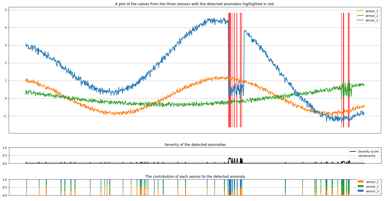
プロットには、センサー (推論ウィンドウ内) の生データがオレンジ、緑、青で表示されます。最初の図の赤い縦線は、重要度が minSeverity 以上の検出された異常を示しています。

2 番目のプロットは、検出されたすべての異常の重要度スコアを示し、minSeverity しきい値は赤い点線で示されています。

最後に、最後のプロットには、検出された異常に対する各センサーからのデータの寄与が示されています。これは、各異常の最も可能性の高い原因を診断して理解するのに役立ちます。

次の方法で共有

レシピ: Azure AI サービス - 多変量異常検出

前提条件

セットアップ

Anomaly Detector リソースを作成する

ストレージアカウントリソースを作成する

サービスキーの入力

フィードバック

フィードバック

その他のリソース

次の方法で共有

レシピ: Azure AI サービス - 多変量異常検出

前提条件

セットアップ

Anomaly Detector リソースを作成する

ストレージ アカウント リソースを作成する

サービス キーの入力

関連するコンテンツ

フィードバック

フィードバック

その他のリソース

ストレージアカウントリソースを作成する

サービスキーの入力