Excel の条件付き書式は、特定の条件またはルールに基づいてセルに書式設定を適用します。 これらの形式は、データが変更されたときに自動的に調整されるため、スクリプトを複数回実行する必要はありません。 このページには、さまざまな条件付き書式オプションを示す Office スクリプトのコレクションが含まれています。
このサンプル ブックには、サンプル スクリプトでテストする準備ができているワークシートが含まれています。
注:
Office スクリプト コード エディターからこれらのサンプルを直接実行します。 コード エディターを開くには、コード エディター で Automate>New Script>Create に移動します。 既定のコードを実行するサンプル コードに置き換え、[ 実行] を選択します。
セルの値
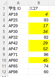
セル値の条件付き書式 は、指定された条件を満たす値を含むすべてのセルに書式を適用します。 これは、重要なデータ ポイントをすばやく見つけるのに役立ちます。
次の例では、セル値の条件付き書式を範囲に適用します。 値が 60 未満の場合、セルの塗りつぶしの色が変更され、フォントが斜体になります。
function main(workbook: ExcelScript.Workbook) {
    // Get the range to format.
    const sheet = workbook.getWorksheet("CellValue");
    const ratingColumn = sheet.getRange("B2:B12");
    sheet.activate();

    // Add cell value conditional formatting.
    const cellValueConditionalFormatting =
        ratingColumn.addConditionalFormat(ExcelScript.ConditionalFormatType.cellValue).getCellValue();

    // Create the condition, in this case when the cell value is less than 60
    let rule: ExcelScript.ConditionalCellValueRule = {
        formula1: "60",
        operator: ExcelScript.ConditionalCellValueOperator.lessThan
    };
    cellValueConditionalFormatting.setRule(rule);

    // Set the format to apply when the condition is met.
    let format = cellValueConditionalFormatting.getFormat();
    format.getFill().setColor("yellow");
    format.getFont().setItalic(true);
}
カラー スケール
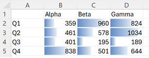
色スケールの条件付き書式は 、範囲全体に色グラデーションを適用します。 範囲の最小値と最大値を持つセルでは、指定された色が使用され、他のセルは比例してスケーリングされます。 オプションの中間点の色は、より多くのコントラストを提供します。
次の例では、選択した範囲に赤、白、青のカラー スケールを適用します。

function main(workbook: ExcelScript.Workbook) {
    // Get the range to format.
    const sheet = workbook.getWorksheet("ColorScale");
    const dataRange = sheet.getRange("B2:M13");
    sheet.activate();

    // Create a new conditional formatting object by adding one to the range.
    const conditionalFormatting = dataRange.addConditionalFormat(ExcelScript.ConditionalFormatType.colorScale);

    // Set the colors for the three parts of the scale: minimum, midpoint, and maximum.
    conditionalFormatting.getColorScale().setCriteria({
        minimum: {
            color: "#5A8AC6", /* A pale blue. */
            type: ExcelScript.ConditionalFormatColorCriterionType.lowestValue
        },
        midpoint: {
            color: "#FCFCFF", /* Slightly off-white. */
            formula: '=50', type: ExcelScript.ConditionalFormatColorCriterionType.percentile
        },
        maximum: {
            color: "#F8696B", /* A pale red. */
            type: ExcelScript.ConditionalFormatColorCriterionType.highestValue
        }
    });
}
データ バー
データ バーの条件付き書式では 、セルの背景に部分的に塗りつぶされたバーが追加されます。 バーの完全性は、セル内の値と、形式で指定された範囲によって定義されます。
次の例では、選択した範囲にデータ バーの条件付き書式を作成します。 データ バーのスケールは 0 から 1200 になります。
function main(workbook: ExcelScript.Workbook) {
    // Get the range to format.
    const sheet = workbook.getWorksheet("DataBar");
    const dataRange = sheet.getRange("B2:D5");
    sheet.activate();

    // Create new conditional formatting on the range.
    const format = dataRange.addConditionalFormat(ExcelScript.ConditionalFormatType.dataBar);
    const dataBarFormat = format.getDataBar();

    // Set the lower bound of the data bar formatting to be 0.
    const lowerBound: ExcelScript.ConditionalDataBarRule = {
        type: ExcelScript.ConditionalFormatRuleType.number,
        formula: "0"
    };
    dataBarFormat.setLowerBoundRule(lowerBound);

    // Set the upper bound of the data bar formatting to be 1200.
    const upperBound: ExcelScript.ConditionalDataBarRule = {
        type: ExcelScript.ConditionalFormatRuleType.number,
        formula: "1200"
    };
    dataBarFormat.setUpperBoundRule(upperBound);
}
アイコン セット
アイコン セットの条件付き書式は、 範囲内の各セルにアイコンを追加します。 アイコンは、指定したセットから取得されます。 アイコンは、条件の順序付けられた配列に基づいて適用され、各条件は 1 つのアイコンにマッピングされます。
次の例では、条件付き書式を範囲に設定する "3 つの信号" アイコンを適用します。
![]()
function main(workbook: ExcelScript.Workbook) {
    // Get the range to format.
    const sheet = workbook.getWorksheet("IconSet");
    const dataRange = sheet.getRange("B2:B12");
    sheet.activate();

    // Create icon set conditional formatting on the range.
    const conditionalFormatting = dataRange.addConditionalFormat(ExcelScript.ConditionalFormatType.iconSet);

    // Use the "3 Traffic Lights (Unrimmed)" set.
    conditionalFormatting.getIconSet().setStyle(ExcelScript.IconSet.threeTrafficLights1);
    conditionalFormatting.getIconSet().setCriteria([
      { // Use the red light as the default for positive values.
        formula: '=0', operator: ExcelScript.ConditionalIconCriterionOperator.greaterThanOrEqual,
        type: ExcelScript.ConditionalFormatIconRuleType.number
      },
      { // The yellow light is applied to all values 6 and greater. The replaces the red light when applicable.
        formula: '=6', operator: ExcelScript.ConditionalIconCriterionOperator.greaterThanOrEqual,
        type: ExcelScript.ConditionalFormatIconRuleType.number
      },
      { // The green light is applied to all values 8 and greater. As with the yellow light, the icon is replaced when the new criteria is met.
        formula: '=8', operator: ExcelScript.ConditionalIconCriterionOperator.greaterThanOrEqual,
        type: ExcelScript.ConditionalFormatIconRuleType.number
      }
    ]);
}
プリセット
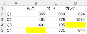
事前設定された条件付き書式 は、空白のセルや重複する値などの一般的なシナリオに基づいて、指定した書式を範囲に適用します。 事前設定された条件の完全な一覧は、 ConditionalFormatPresetCriterion 列挙型によって提供されます。
次の例では、範囲内の空白セルに黄色の塗りつぶしを指定します。
function main(workbook: ExcelScript.Workbook) {
    // Get the range to format.
    const sheet = workbook.getWorksheet("Preset");
    const dataRange = sheet.getRange("B2:D5");
    sheet.activate();

    // Add new conditional formatting to that range.
    const conditionalFormat = dataRange.addConditionalFormat(
    ExcelScript.ConditionalFormatType.presetCriteria);

    // Set the conditional formatting to apply a yellow fill.
    const presetFormat = conditionalFormat.getPreset();
    presetFormat.getFormat().getFill().setColor("yellow");

    // Set a rule to apply the conditional format when cells are left blank.
    const blankRule: ExcelScript.ConditionalPresetCriteriaRule = {
        criterion: ExcelScript.ConditionalFormatPresetCriterion.blanks
    };
    presetFormat.setRule(blankRule);
}
テキストの比較
テキスト比較の条件付き書式は、 セルのテキスト コンテンツに基づいて書式設定します。 書式設定は、テキストがで始まる、含む、で終わる、または指定された部分文字列が含まれていない場合に適用されます。
次の例では、"review" というテキストを含む範囲内のセルをマークします。

function main(workbook: ExcelScript.Workbook) {
    // Get the range to format.
    const sheet = workbook.getWorksheet("TextComparison");
    const dataRange = sheet.getRange("B2:B6");
    sheet.activate();

    // Add conditional formatting based on the text in the cells.
    const textConditionFormat = dataRange.addConditionalFormat(
        ExcelScript.ConditionalFormatType.containsText).getTextComparison();

    // Set the conditional format to provide a light red fill and make the font bold.
    textConditionFormat.getFormat().getFill().setColor("#F8696B");
    textConditionFormat.getFormat().getFont().setBold(true);

    // Apply the condition rule that the text contains with "review".
    const textRule: ExcelScript.ConditionalTextComparisonRule = {
        operator: ExcelScript.ConditionalTextOperator.contains,
        text: "review"
    };
    textConditionFormat.setRule(textRule);
}
上/下
上/下の条件付き書式は 、範囲内の最大値または最小値をマークします。 高値と安値は、生の値またはパーセンテージに基づいています。
次の例では、条件付き書式を適用して、範囲内で最も高い 2 つの数値を表示します。
function main(workbook: ExcelScript.Workbook) {
  // Get the range to format.
  const sheet = workbook.getWorksheet("TopBottom");
  const dataRange = sheet.getRange("B2:D5");
  sheet.activate();

    // Set the fill color to green and the font to bold for the top 2 values in the range.
    const topBottomFormat = dataRange.addConditionalFormat(ExcelScript.ConditionalFormatType.topBottom).getTopBottom();
    topBottomFormat.getFormat().getFill().setColor("green");
    topBottomFormat.getFormat().getFont().setBold(true);
    topBottomFormat.setRule({
      rank: 2, /* The numeric threshold. */
      type: ExcelScript.ConditionalTopBottomCriterionType.topItems /* The type of the top/bottom condition. */
    });
}
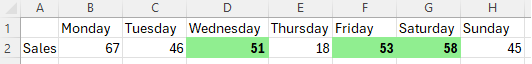
カスタム条件
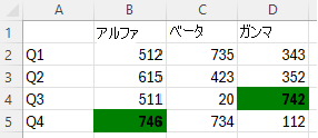
カスタム条件付き書式を 使用すると、書式設定を適用するタイミングを複雑な数式で定義できます。 他のオプションで十分でない場合は、これを使用します。
次の例では、選択した範囲にカスタムの条件付き書式を設定します。 値が行の前の列の値より大きい場合は、明るい緑色の塗りつぶしと太字のフォントがセルに適用されます。
function main(workbook: ExcelScript.Workbook) {
    // Get the range to format.
    const sheet = workbook.getWorksheet("Custom");
    const dataRange = sheet.getRange("B2:H2");
    sheet.activate();

    // Apply a rule for positive change from the previous column.
    const positiveChange = dataRange.addConditionalFormat(ExcelScript.ConditionalFormatType.custom).getCustom();
    positiveChange.getFormat().getFill().setColor("lightgreen");
    positiveChange.getFormat().getFont().setBold(true);
    positiveChange.getRule().setFormula(
        `=${dataRange.getCell(0, 0).getAddress()}>${dataRange.getOffsetRange(0, -1).getCell(0, 0).getAddress()}`
    );
}
GitHub で Microsoft と共同作業する
このコンテンツのソースは GitHub にあります。そこで、issue や pull request を作成および確認することもできます。 詳細については、共同作成者ガイドを参照してください。
Office Scripts