演習 - 実際の問題のリソースを推定する - Training

10 分

Shor の因数分解アルゴリズムは、最もよく知られている量子アルゴリズムの 1 つです。これは、既知の古典的な因数分解アルゴリズムに対して指数関数的な高速化を提供します。

古典的な暗号は、計算の困難性など、物理的または数学的な手段を使用してタスクを実行します。一般的な暗号化プロトコルは Rivest-Shamir-Adleman (RSA) スキームであり、これは、古典的コンピューターを使用した素因数分解が困難であるという仮定に基づいています。

Shor のアルゴリズムは、十分に大きい量子コンピューターが公開鍵暗号を解読できることを示唆しています。これらの種類の暗号化スキームの脆弱性を評価するには、ショアのアルゴリズムに必要なリソースの推定が重要です。

次の演習では、2048 ビットの整数の素因数分解のリソース推定を計算します。このアプリケーションでは、あらかじめ計算されている論理リソースの見積もりから物理リソースの見積もりを直接計算します。許容されるエラーバジェットには、$\epsilon = 1/3$ を使用します。

Shor のアルゴリズムを記述する

VS Code で、[表示] > [コマンドパレット] を選択して、[作成: 新しい Jupyter Notebook] を選択します。
ノートブックを ShorRE.ipynb として保存します。
ノートブックの最初のセルで、qsharp パッケージをインポートします。
```
import qsharp
```

Microsoft.Quantum.ResourceEstimation 名前空間を使用して、Shor の素因数分解アルゴリズムのキャッシュされた最適化バージョンを定義します。新しいセルを追加して次のコードをコピーします。

%%qsharp
open Microsoft.Quantum.Arrays;
open Microsoft.Quantum.Canon;
open Microsoft.Quantum.Convert;
open Microsoft.Quantum.Diagnostics;
open Microsoft.Quantum.Intrinsic;
open Microsoft.Quantum.Math;
open Microsoft.Quantum.Measurement;
open Microsoft.Quantum.Unstable.Arithmetic;
open Microsoft.Quantum.ResourceEstimation;

operation RunProgram() : Unit {
    let bitsize = 31;

    // When choosing parameters for `EstimateFrequency`, make sure that
    // generator and modules are not co-prime
    let _ = EstimateFrequency(11, 2^bitsize - 1, bitsize);
}


// In this sample we concentrate on costing the `EstimateFrequency`
// operation, which is the core quantum operation in Shors algorithm, and
// we omit the classical pre- and post-processing.

/// # Summary
/// Estimates the frequency of a generator
/// in the residue ring Z mod `modulus`.
///
/// # Input
/// ## generator
/// The unsigned integer multiplicative order (period)
/// of which is being estimated. Must be co-prime to `modulus`.
/// ## modulus
/// The modulus which defines the residue ring Z mod `modulus`
/// in which the multiplicative order of `generator` is being estimated.
/// ## bitsize
/// Number of bits needed to represent the modulus.
///
/// # Output
/// The numerator k of dyadic fraction k/2^bitsPrecision
/// approximating s/r.
operation EstimateFrequency(
    generator : Int,
    modulus : Int,
    bitsize : Int
)
: Int {
    mutable frequencyEstimate = 0;
    let bitsPrecision =  2 * bitsize + 1;

    // Allocate qubits for the superposition of eigenstates of
    // the oracle that is used in period finding.
    use eigenstateRegister = Qubit[bitsize];

    // Initialize eigenstateRegister to 1, which is a superposition of
    // the eigenstates we are estimating the phases of.
    // We first interpret the register as encoding an unsigned integer
    // in little endian encoding.
    ApplyXorInPlace(1, eigenstateRegister);
    let oracle = ApplyOrderFindingOracle(generator, modulus, _, _);

    // Use phase estimation with a semiclassical Fourier transform to
    // estimate the frequency.
    use c = Qubit();
    for idx in bitsPrecision - 1..-1..0 {
        within {
            H(c);
        } apply {
            // `BeginEstimateCaching` and `EndEstimateCaching` are the operations
            // exposed by Azure Quantum Resource Estimator. These will instruct
            // resource counting such that the if-block will be executed
            // only once, its resources will be cached, and appended in
            // every other iteration.
            if BeginEstimateCaching("ControlledOracle", SingleVariant()) {
                Controlled oracle([c], (1 <<< idx, eigenstateRegister));
                EndEstimateCaching();
            }
            R1Frac(frequencyEstimate, bitsPrecision - 1 - idx, c);
        }
        if MResetZ(c) == One {
            set frequencyEstimate += 1 <<< (bitsPrecision - 1 - idx);
        }
    }

    // Return all the qubits used for oracles eigenstate back to 0 state
    // using Microsoft.Quantum.Intrinsic.ResetAll.
    ResetAll(eigenstateRegister);

    return frequencyEstimate;
}

/// # Summary
/// Interprets `target` as encoding unsigned little-endian integer k
/// and performs transformation |k⟩ ↦ |gᵖ⋅k mod N ⟩ where
/// p is `power`, g is `generator` and N is `modulus`.
///
/// # Input
/// ## generator
/// The unsigned integer multiplicative order ( period )
/// of which is being estimated. Must be co-prime to `modulus`.
/// ## modulus
/// The modulus which defines the residue ring Z mod `modulus`
/// in which the multiplicative order of `generator` is being estimated.
/// ## power
/// Power of `generator` by which `target` is multiplied.
/// ## target
/// Register interpreted as LittleEndian which is multiplied by
/// given power of the generator. The multiplication is performed modulo
/// `modulus`.
internal operation ApplyOrderFindingOracle(
    generator : Int, modulus : Int, power : Int, target : Qubit[]
)
: Unit
is Adj + Ctl {
    // The oracle we use for order finding implements |x⟩ ↦ |x⋅a mod N⟩. We
    // also use `ExpModI` to compute a by which x must be multiplied. Also
    // note that we interpret target as unsigned integer in little-endian
    // encoding by using the `LittleEndian` type.
    ModularMultiplyByConstant(modulus,
                                ExpModI(generator, power, modulus),
                                target);
}

/// # Summary
/// Performs modular in-place multiplication by a classical constant.
///
/// # Description
/// Given the classical constants `c` and `modulus`, and an input
/// quantum register (as LittleEndian) |𝑦⟩, this operation
/// computes `(c*x) % modulus` into |𝑦⟩.
///
/// # Input
/// ## modulus
/// Modulus to use for modular multiplication
/// ## c
/// Constant by which to multiply |𝑦⟩
/// ## y
/// Quantum register of target
internal operation ModularMultiplyByConstant(modulus : Int, c : Int, y : Qubit[])
: Unit is Adj + Ctl {
    use qs = Qubit[Length(y)];
    for (idx, yq) in Enumerated(y) {
        let shiftedC = (c <<< idx) % modulus;
        Controlled ModularAddConstant([yq], (modulus, shiftedC, qs));
    }
    ApplyToEachCA(SWAP, Zipped(y, qs));
    let invC = InverseModI(c, modulus);
    for (idx, yq) in Enumerated(y) {
        let shiftedC = (invC <<< idx) % modulus;
        Controlled ModularAddConstant([yq], (modulus, modulus - shiftedC, qs));
    }
}

/// # Summary
/// Performs modular in-place addition of a classical constant into a
/// quantum register.
///
/// # Description
/// Given the classical constants `c` and `modulus`, and an input
/// quantum register (as LittleEndian) |𝑦⟩, this operation
/// computes `(x+c) % modulus` into |𝑦⟩.
///
/// # Input
/// ## modulus
/// Modulus to use for modular addition
/// ## c
/// Constant to add to |𝑦⟩
/// ## y
/// Quantum register of target
internal operation ModularAddConstant(modulus : Int, c : Int, y : Qubit[])
: Unit is Adj + Ctl {
    body (...) {
        Controlled ModularAddConstant([], (modulus, c, y));
    }
    controlled (ctrls, ...) {
        // We apply a custom strategy to control this operation instead of
        // letting the compiler create the controlled variant for us in which
        // the `Controlled` functor would be distributed over each operation
        // in the body.
        //
        // Here we can use some scratch memory to save ensure that at most one
        // control qubit is used for costly operations such as `AddConstant`
        // and `CompareGreaterThenOrEqualConstant`.
        if Length(ctrls) >= 2 {
            use control = Qubit();
            within {
                Controlled X(ctrls, control);
            } apply {
                Controlled ModularAddConstant([control], (modulus, c, y));
            }
        } else {
            use carry = Qubit();
            Controlled AddConstant(ctrls, (c, y + [carry]));
            Controlled Adjoint AddConstant(ctrls, (modulus, y + [carry]));
            Controlled AddConstant([carry], (modulus, y));
            Controlled CompareGreaterThanOrEqualConstant(ctrls, (c, y, carry));
        }
    }
}

/// # Summary
/// Performs in-place addition of a constant into a quantum register.
///
/// # Description
/// Given a non-empty quantum register |𝑦⟩ of length 𝑛+1 and a positive
/// constant 𝑐 < 2ⁿ, computes |𝑦 + c⟩ into |𝑦⟩.
///
/// # Input
/// ## c
/// Constant number to add to |𝑦⟩.
/// ## y
/// Quantum register of second summand and target; must not be empty.
internal operation AddConstant(c : Int, y : Qubit[]) : Unit is Adj + Ctl {
    // We are using this version instead of the library version that is based
    // on Fourier angles to show an advantage of sparse simulation in this sample.

    let n = Length(y);
    Fact(n > 0, "Bit width must be at least 1");

    Fact(c >= 0, "constant must not be negative");
    Fact(c < 2 ^ n, $"constant must be smaller than {2L ^ n}");

    if c != 0 {
        // If c has j trailing zeroes than the j least significant bits
        // of y will not be affected by the addition and can therefore be
        // ignored by applying the addition only to the other qubits and
        // shifting c accordingly.
        let j = NTrailingZeroes(c);
        use x = Qubit[n - j];
        within {
            ApplyXorInPlace(c >>> j, x);
        } apply {
            IncByLE(x, y[j...]);
        }
    }
}

/// # Summary
/// Performs greater-than-or-equals comparison to a constant.
///
/// # Description
/// Toggles output qubit `target` if and only if input register `x`
/// is greater than or equal to `c`.
///
/// # Input
/// ## c
/// Constant value for comparison.
/// ## x
/// Quantum register to compare against.
/// ## target
/// Target qubit for comparison result.
///
/// # Reference
/// This construction is described in [Lemma 3, arXiv:2201.10200]
internal operation CompareGreaterThanOrEqualConstant(c : Int, x : Qubit[], target : Qubit)
: Unit is Adj+Ctl {
    let bitWidth = Length(x);

    if c == 0 {
        X(target);
    } elif c >= 2 ^ bitWidth {
        // do nothing
    } elif c == 2 ^ (bitWidth - 1) {
        ApplyLowTCNOT(Tail(x), target);
    } else {
        // normalize constant
        let l = NTrailingZeroes(c);

        let cNormalized = c >>> l;
        let xNormalized = x[l...];
        let bitWidthNormalized = Length(xNormalized);
        let gates = Rest(IntAsBoolArray(cNormalized, bitWidthNormalized));

        use qs = Qubit[bitWidthNormalized - 1];
        let cs1 = [Head(xNormalized)] + Most(qs);
        let cs2 = Rest(xNormalized);

        within {
            for i in IndexRange(gates) {
                (gates[i] ? ApplyAnd | ApplyOr)(cs1[i], cs2[i], qs[i]);
            }
        } apply {
            ApplyLowTCNOT(Tail(qs), target);
        }
    }
}

/// # Summary
/// Internal operation used in the implementation of GreaterThanOrEqualConstant.
internal operation ApplyOr(control1 : Qubit, control2 : Qubit, target : Qubit) : Unit is Adj {
    within {
        ApplyToEachA(X, [control1, control2]);
    } apply {
        ApplyAnd(control1, control2, target);
        X(target);
    }
}

internal operation ApplyAnd(control1 : Qubit, control2 : Qubit, target : Qubit)
: Unit is Adj {
    body (...) {
        CCNOT(control1, control2, target);
    }
    adjoint (...) {
        H(target);
        if (M(target) == One) {
            X(target);
            CZ(control1, control2);
        }
    }
}


/// # Summary
/// Returns the number of trailing zeroes of a number
///
/// ## Example
/// ```qsharp
/// let zeroes = NTrailingZeroes(21); // = NTrailingZeroes(0b1101) = 0
/// let zeroes = NTrailingZeroes(20); // = NTrailingZeroes(0b1100) = 2
/// ```
internal function NTrailingZeroes(number : Int) : Int {
    mutable nZeroes = 0;
    mutable copy = number;
    while (copy % 2 == 0) {
        set nZeroes += 1;
        set copy /= 2;
    }
    return nZeroes;
}

/// # Summary
/// An implementation for `CNOT` that when controlled using a single control uses
/// a helper qubit and uses `ApplyAnd` to reduce the T-count to 4 instead of 7.
internal operation ApplyLowTCNOT(a : Qubit, b : Qubit) : Unit is Adj+Ctl {
    body (...) {
        CNOT(a, b);
    }

    adjoint self;

    controlled (ctls, ...) {
        // In this application this operation is used in a way that
        // it is controlled by at most one qubit.
        Fact(Length(ctls) <= 1, "At most one control line allowed");

        if IsEmpty(ctls) {
            CNOT(a, b);
        } else {
            use q = Qubit();
            within {
                ApplyAnd(Head(ctls), a, q);
            } apply {
                CNOT(q, b);
            }
        }
    }

    controlled adjoint self;
}

Shor のアルゴリズムの推定を行う

次に、既定の前提条件を使用して RunProgram 操作の物理リソースを推定します。新しいセルを追加して次のコードをコピーします。

result = qsharp.estimate("RunProgram()")
result

qsharp.estimate 関数は結果オブジェクトを作成し、これは全体的な物理リソースの総数を含むテーブルを表示するために使用できます。詳しい情報が含まれているグループを折りたたんで、コストの詳細を確認できます。

たとえば、論理量子ビットパラメーター グループを折りたたんで、符号距離が 21 で、物理量子ビットの数が 882 であることを確認します。

論理量子ビットパラメーター	Value
QEC スキーム	surface_code
コード距離	21
物理量子ビット	882
論理サイクル時間	8 ミリ秒
論理量子ビットエラー率	3.00E-13
交差の前因子	0.03
エラー訂正のしきい値	0.01
論理サイクル時間の数式	(4 * `twoQubitGateTime` + 2 * `oneQubitMeasurementTime`) * `codeDistance`
物理量子ビットの数式	2 * `codeDistance` * `codeDistance`

ヒント

よりコンパクトなバージョンの出力テーブルが必要であれば、result.summary を使用できます。

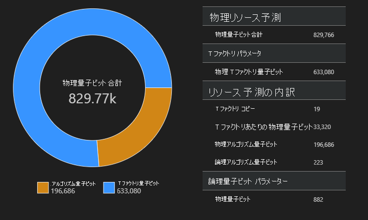
空間図

アルゴリズムと T ファクトリに使用される物理量子ビットの分布は、アルゴリズムの設計に影響を与える可能性のある要因です。 qsharp-widgets パッケージを使用してこの分布を視覚化すると、アルゴリズムの推定される空間的要件をより深く理解できます。

from qsharp_widgets import SpaceChart
SpaceChart(result)

この例では、アルゴリズムを実行するために必要な物理量子ビットの数は 829766 であり、そのうちの 196686 個がアルゴリズム量子ビットであり、633080 個が T ファクトリ量子ビットです。

Screenshot showing the space diagram of the Resource Estimator.

さまざまな量子ビットテクノロジのリソース見積もりを比較する

Azure Quantum Resource Estimator を使用すると、ターゲットパラメーターの複数の構成を実行し、結果を比較できます。これはさまざまな量子ビットモデル、QEC スキーム、またはエラーバジェットのコストを比較したい場合に便利です。

EstimatorParams オブジェクトを使用して推定パラメーターの一覧を作成することもできます。

from qsharp.estimator import EstimatorParams, QubitParams, QECScheme, LogicalCounts

labels = ["Gate-based µs, 10⁻³", "Gate-based µs, 10⁻⁴", "Gate-based ns, 10⁻³", "Gate-based ns, 10⁻⁴", "Majorana ns, 10⁻⁴", "Majorana ns, 10⁻⁶"]

params = EstimatorParams(6)
params.error_budget = 0.333
params.items[0].qubit_params.name = QubitParams.GATE_US_E3
params.items[1].qubit_params.name = QubitParams.GATE_US_E4
params.items[2].qubit_params.name = QubitParams.GATE_NS_E3
params.items[3].qubit_params.name = QubitParams.GATE_NS_E4
params.items[4].qubit_params.name = QubitParams.MAJ_NS_E4
params.items[4].qec_scheme.name = QECScheme.FLOQUET_CODE
params.items[5].qubit_params.name = QubitParams.MAJ_NS_E6
params.items[5].qec_scheme.name = QECScheme.FLOQUET_CODE

qsharp.estimate("RunProgram()", params=params).summary_data_frame(labels=labels)

量子ビットモデル	論理量子ビット	論理的な深さ	T 状態	コード距離	T ファクトリ	T ファクトリ小数	物理量子ビット	rQOPS	物理ランタイム
ゲートベースの µs、10⁻³	223 3.64M	4.70M	17	13	40.54 %	216.77k	21.86k	10 時間
ゲートベースの µs、10⁻⁴	223	3.64M	4.70M	9	14	43.17 %	63.57k	41.30k	5 時間
ゲートベースの ns、10⁻³	223 3.64M	4.70M	17	16	69.08 %	416.89k	32.79M	25 秒
ゲートベースの ns、10⁻⁴	223 3.64M	4.70M	9	14	43.17 %	63.57k	61.94M	13 秒
Majorana の ns、10⁻⁴	223 3.64M	4.70M	9	19	82.75 %	501.48k	82.59M	10 秒
Majorana の ns、10⁻⁶	223 3.64M	4.70M	5	13	31.47 %	42.96k	148.67M	5 秒

論理リソース数からリソース推定を抽出する

操作について既にわかっている見積もりがある場合は、リソース推定器を使ってプログラムの全体的なコストに既知の見積もりを組み込んで、実行時間を短縮できます。 LogicalCounts クラスを使用して、事前に計算されたリソース見積もり値から論理リソース見積もりを抽出できます。

[コード] を選択して新しいセルを追加し、次のコードを入力して実行してください。

logical_counts = LogicalCounts({
    'numQubits': 12581,
    'tCount': 12,
    'rotationCount': 12,
    'rotationDepth': 12,
    'cczCount': 3731607428,
    'measurementCount': 1078154040})

logical_counts.estimate(params).summary_data_frame(labels=labels)

量子ビットモデル	論理量子ビット	論理的な深さ	T 状態	コード距離	T ファクトリ	T ファクトリ小数	物理量子ビット	物理ランタイム
ゲートベースの µs、10⁻³	25481	1.2e+10	1.5e+10	27	13	0.6%	37.38M	6 年
ゲートベースの µs、10⁻⁴	25481	1.2e+10	1.5e+10	13	14	0.8%	8.68M	3 年
ゲートベースの ns、10⁻³	25481	1.2e+10	1.5e+10	27	15	1.3%	37.65M	2 日
ゲートベースの ns、10⁻⁴	25481	1.2e+10	1.5e+10	13	18	1.2%	8.72M	18 時間
Majorana の ns、10⁻⁴	25481	1.2e+10	1.5e+10	15	15	1.3%	26.11M	15 時間
Majorana の ns、10⁻⁶	25481	1.2e+10	1.5e+10	7	13	0.5%	6.25M	7 時間

まとめ

最悪のシナリオでは、ゲートベースの µs 量子ビット (超伝導量子ビットなどのナノ秒領域の演算時間を持つ量子ビット) と表面 QEC 符号を使用する量子コンピューターは、Shor のアルゴリズムを使用して 2048 ビットの整数を素因数分解するのに 6 年と 3,738 万の量子ビットを必要することになります。

ゲートベースの ns イオン量子ビットと同じ surface code など、別の量子ビットテクノロジを使用する場合、量子ビットの数はあまり変わりませんが、ランタイムは最悪の場合で 2 日、楽観的な場合で 18 時間になりました。たとえば、Majorana ベースの量子ビットを使用して量子ビットテクノロジと QEC コードを変更した場合、最良のシナリオでは、625 万量子ビットの配列で、ショアのアルゴリズムを使用して 2048 ビットの整数を数時間で素因数分解できます。

実験から、Shor のアルゴリズムを実行して 2048 ビットの整数を素因数分解するには、Majorana 量子ビットと Floquet QEC 符号を使用するのが最善の選択であると結論付けることができます。

続行

演習 - 実際の問題のリソースを推定する

Shor のアルゴリズムを記述する

Shor のアルゴリズムの推定を行う

空間図

さまざまな量子ビット テクノロジのリソース見積もりを比較する

論理リソース数からリソース推定を抽出する

まとめ

フィードバック

さまざまな量子ビットテクノロジのリソース見積もりを比較する