A Practical Example of How to Apply Power Query Data Transformations to Structured and Unstructured Datasets
Introduction
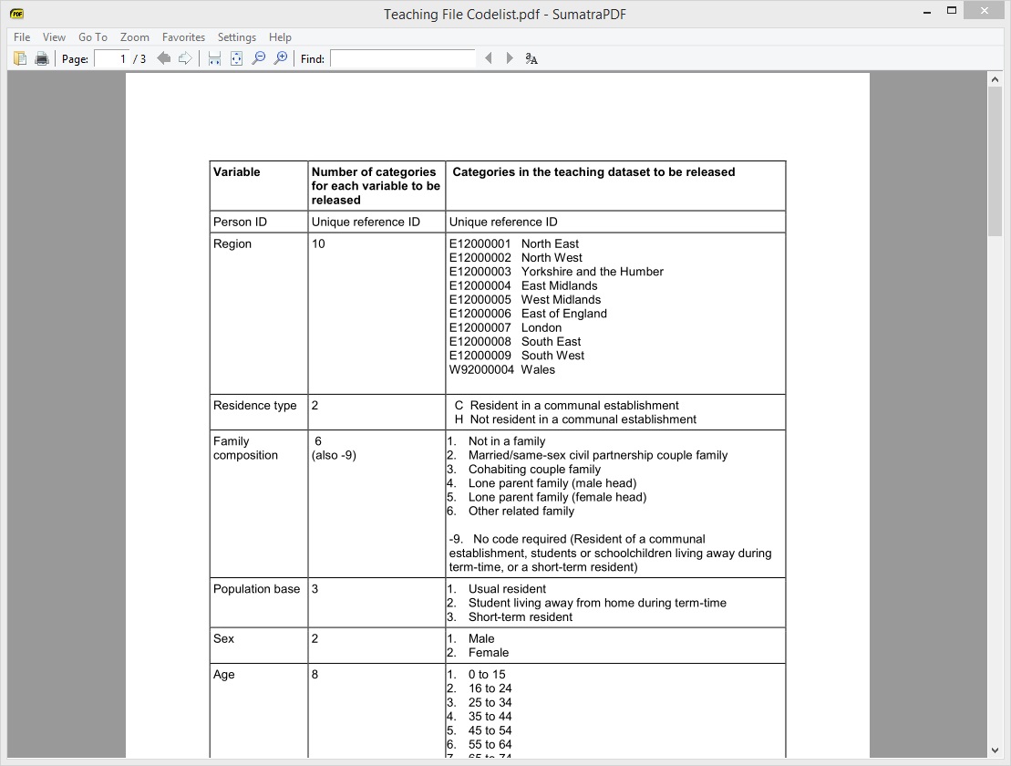
Power Query is a quite a new technology and some of you may want to see an example of how it can be used to transform real data into a shape that's good enough to be consumed by a Power Pivot Data Model. This article will walk you through how Power Query was used to transform and shape UK National Census 2011 data that was publicly released by the Office for National Statistics (ONS) in January 2014. The fact data has been provided in a CSV file, but the look-up/reference data was supplied in a PDF document. We will look at how Power Query was used to transform both the structured and unstructured data into a state that was suitable for modelling in Power Pivot.
The data used in this example is a 1% representative sample of all the UK Census 2011 results. ONS refer to it as a 'Teaching file' and it contains over 500,000 rows of data.

Transforming the structured data
The first thing that needed to be done was to load the data from the CSV file. This was done by selecting the From File > From CSV data loading method found under the Power Query tab...
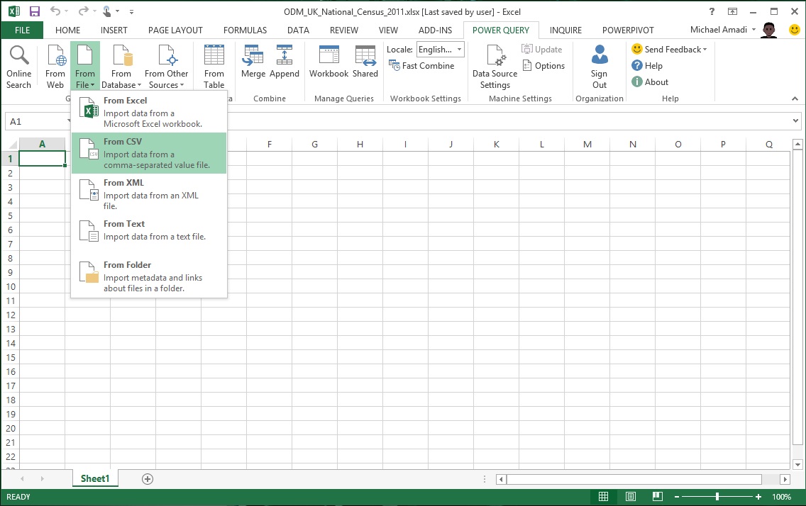
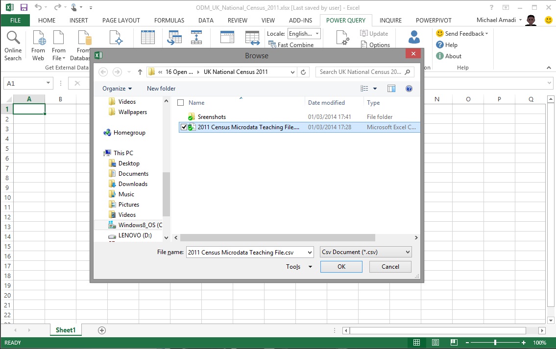
…and then choosing the CSV file.
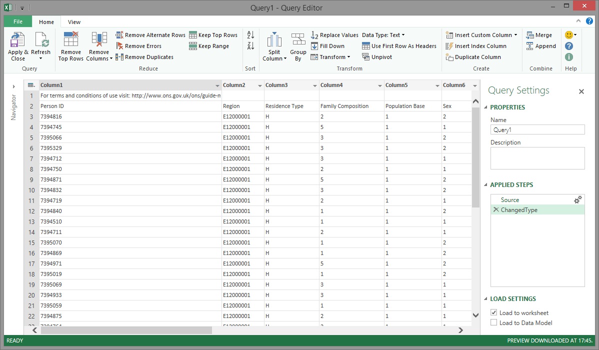
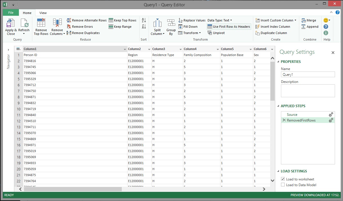
Power Query extracted all of the rows from the CSV file successfully but the data in row 1 wasn't truly part of the dataset and it needed to be removed.
Enter Power Query's Remove Top Rows transformation which allows us to remove unwanted rows starting from the top of the dataset. In this case, only a single row was to be removed and this was done by entering '1' in the Number of rows field before proceeding.
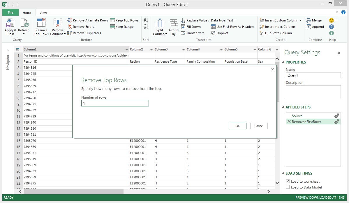
The unwanted row was successfully removed.
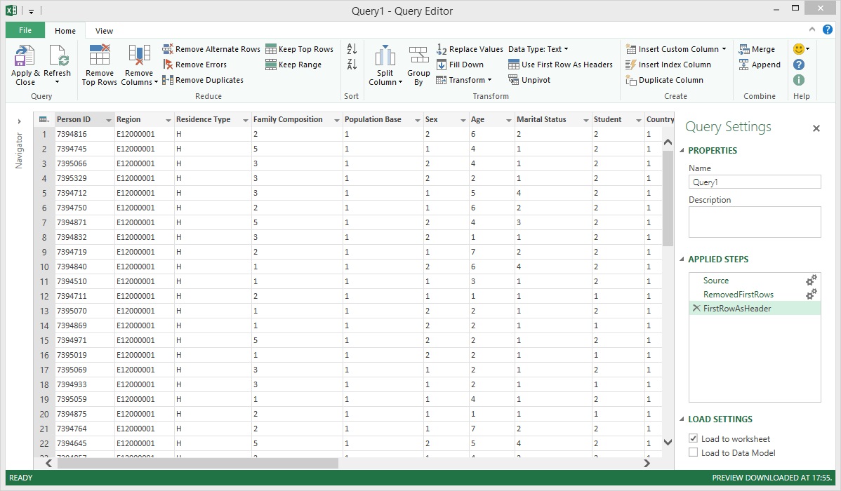
The next problem was that the header row for the dataset was being treated like a data row. To fix this the Use First Row As Headers transformation was applied and, like magic, each column was given the correct heading.
At this point the dataset was nearly good enough to load into Power Pivot but before doing so, the correct data types were set for each column. This was done by selecting each column and then picking the correct data type in the Data Type field. It just so happened that all of the columns except for 'Region' and 'Residence Type' contained numeric data so the Number data type was set for these. Power Query had already selected the Text data type for the 'Region' and 'Residence Type' columns which was correct.
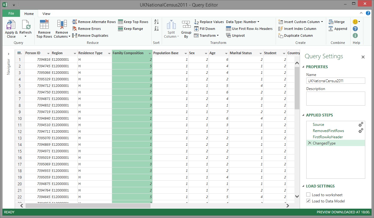
Those of you who have worked with Power Query before or who have been paying close attention to the images have noticed that the Applied Steps list has been getting longer with each data transformation that was applied. You can see in the image above that there is a new step in the Applied Steps list called 'ChangedType'. What's interesting to note is that regardless of whether the column data type was changed one column at a time or several columns were highlighted and changed in one go, a single step was recorded in the Applied Steps list. A very useful feature of Power Query's Applied Steps list is that it can be used to visually see how the data looks before and after a transformation step is applied. It also allows you to amend the transformation in the event that a mistake was made.
At this stage the dataset had been transformed into a structure that was suitable for loading into Power Pivot so it was renamed from 'Query1' to 'UKNationalCensus2011'. It's important to note here that whatever name you give a query here is the same name that will be used for the table when it's created in the Power Pivot Data Model. It's best to choose the name carefully the first time round to avoid having to rename it later and potentially causing issues in your Power Pivot Data Model.
Take another look at the image above and notice that, under the Load Settings area, the Load to worksheet option has been unchecked and the Load to Data Model option has been checked instead. This was done to ensure that Power Query loaded the data directly into the Power Pivot model without the overhead of having to also materialize the data in a worksheet. The only thing left to do at this stage was to click Apply & Close to start loading the data into Power Pivot.
Power Query took under a minute to load the data into Power Pivot.
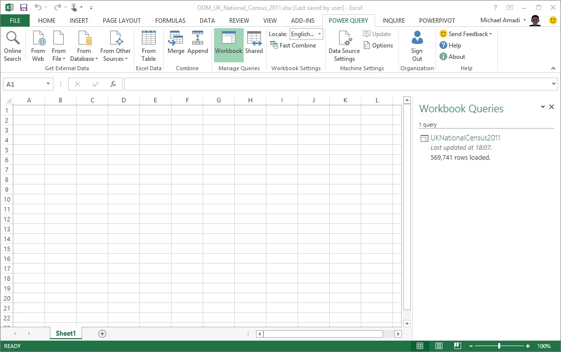
Let's take a quick look at the Power Pivot window.
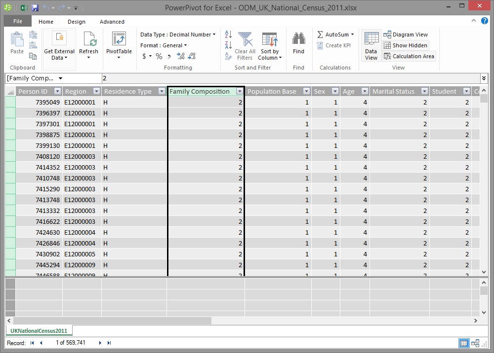
As you can see, the data is all there and the headers are correct. However, there is something a bit strange about the columns that were given the Number data type in Power Query; they have been loaded into Power Pivot with a Decimal Number data type! This is a good time to point out that, by default, columns defined as Number data types** in **Power Query will be loaded into Power Pivot with the Decimal Number data type. If a column will only ever contain whole numbers (i.e. integers) and you are loading them via Power Query, be sure to set them to the Whole Number data type after the table is first loaded into Power Pivot. This will contribute towards a smaller Power Pivot Data Model size and, consequently, a smaller workbook file size. It will also contribute towards a better performing model if the columns are used for aggregation calculations and/or to link tables together.
Transforming the unstructured data
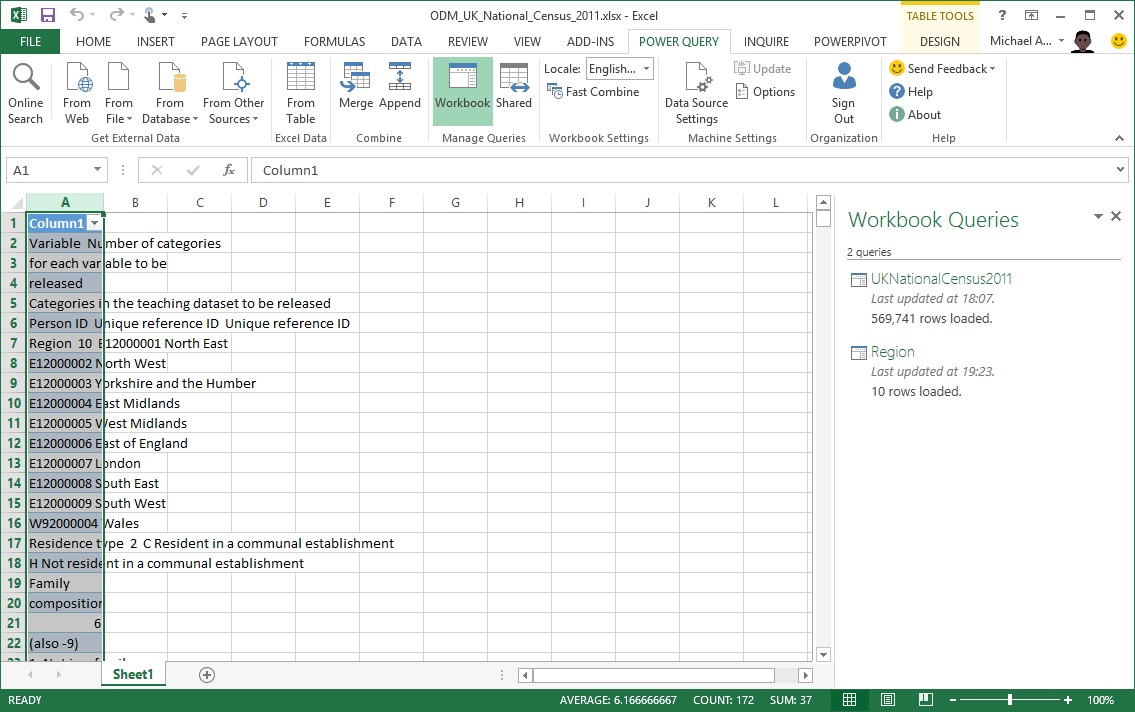
The fact data has been loaded so far but what about the reference tables (i.e. look-up tables)? As this data was stored in a PDF document a slightly different approach was required. The data was copied and pasted from the PDF document into a blank worksheet in the Excel workbook. It's likely that there are 'more clever' ways of getting the data into a format that Power Query can easily read, but this was sufficient in this scenario as the reference data is static.
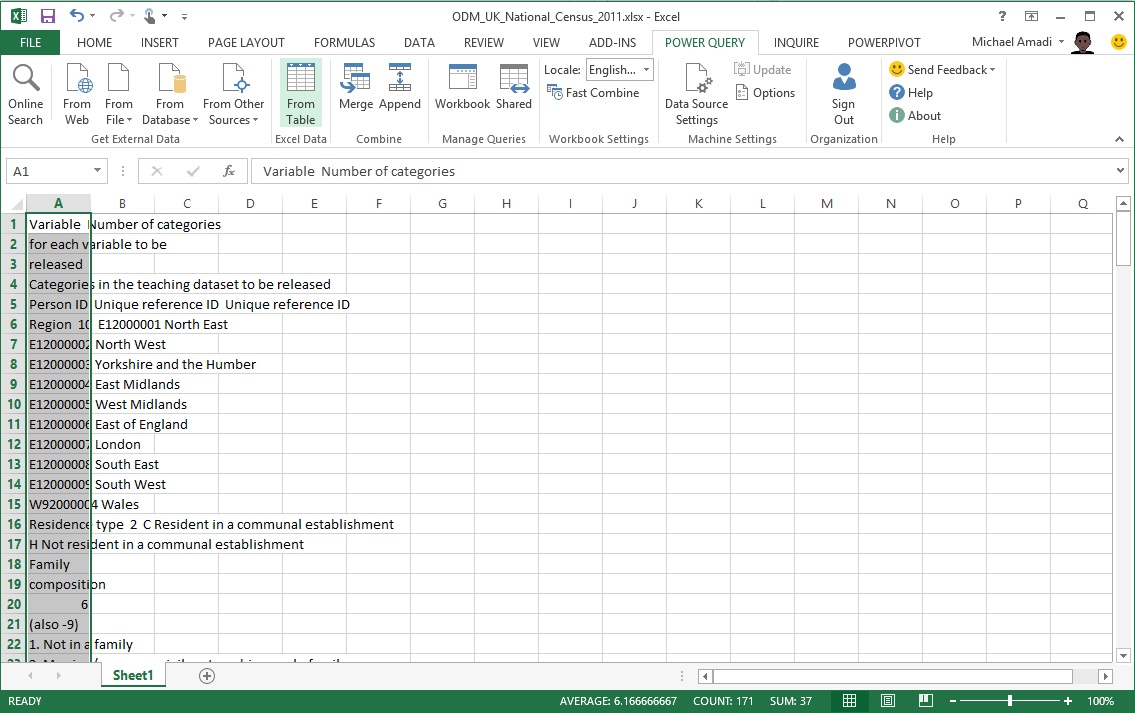
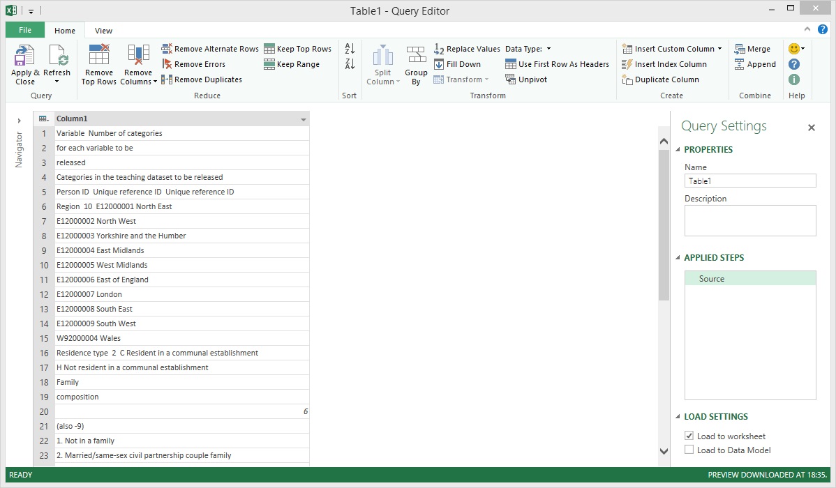
This is what the unstructured data looked like after being pasted into Excel...
Having placed the data into an Excel worksheet, the From Table data loading feature was used. Note that the My table has headers checkbox was unchecked before continuing because the column contained unstructured data.
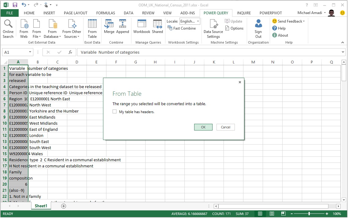
The data was successfully loaded into the Query Editor after clicking OK.
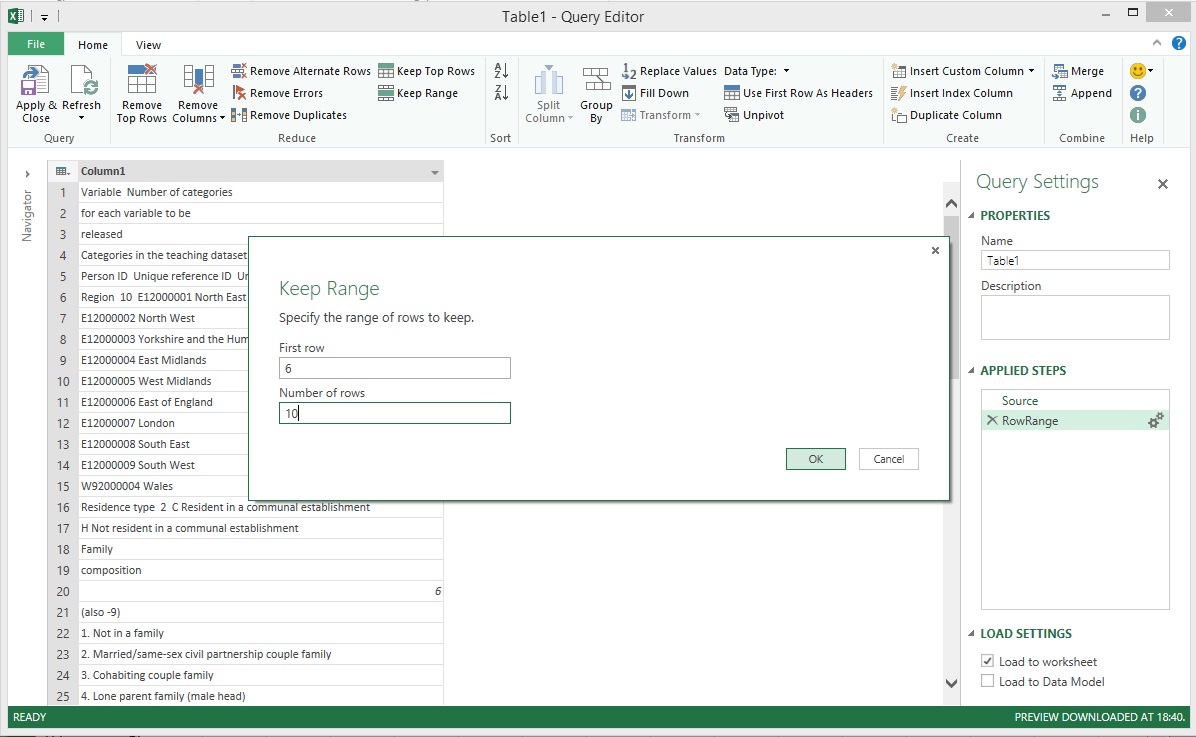
Power Query has a very handy transformation called Keep Range which allows us to get a sub-set of the rows in a table. 'Region' was the first dataset that needed to be extracted from the long list of unstructured data. Take another look at the image above and you will notice that the values for 'Region' start at row 6 and end at row 15. This is why '6' was entered in the First row field. '10' was entered in the Number of rows field because there were only 10 rows of data including row 6 that were part of the region dataset.
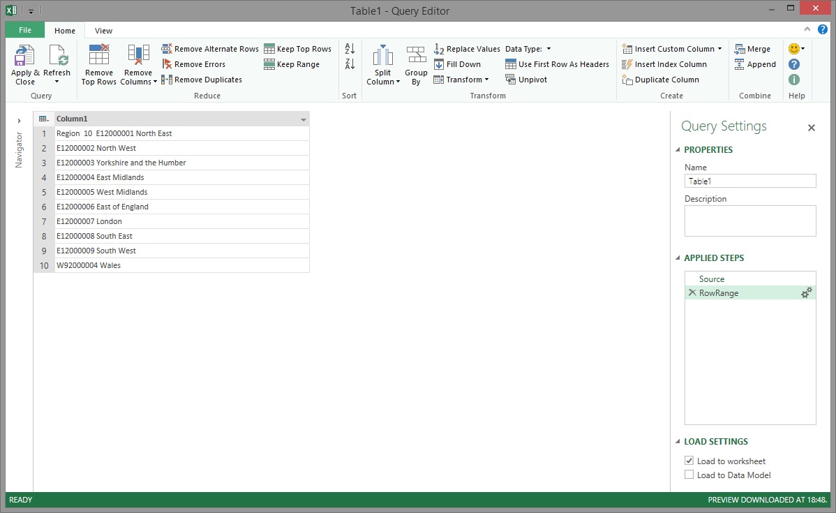
The Power Query magic gave us back 10 rows as expected but there were still a few things that had to be done to this data before it was 'Power Pivot worthy'.
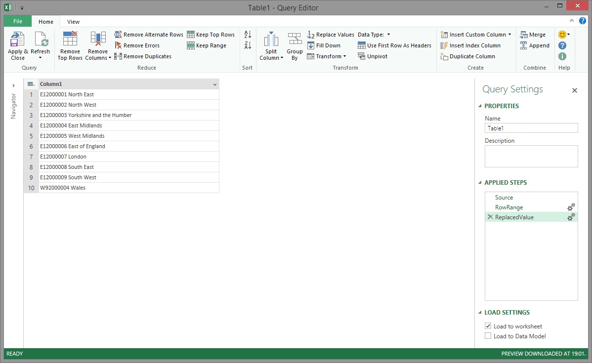
Firstly, the 'Region 10 ' text that preceded the valid data in row 1 needed to be removed and this is where Power Query's Replace Values transformation came into play. The text 'Region 10 ' was entered in the Value To Find before proceeding.
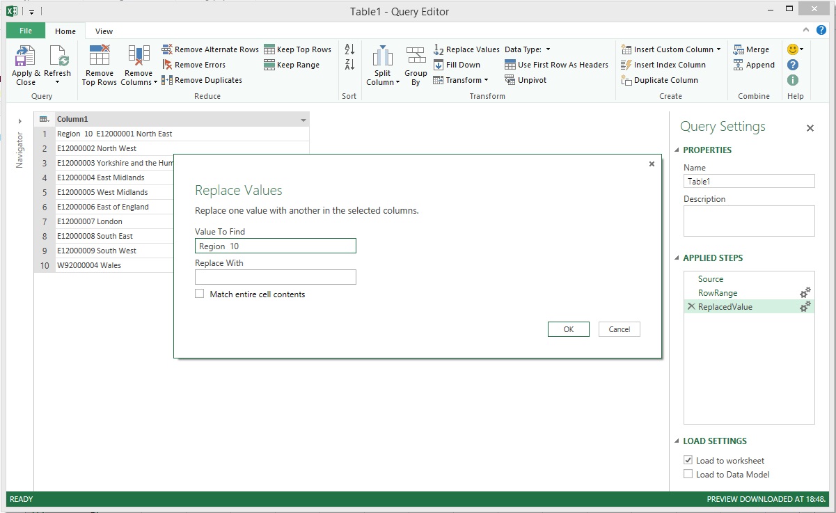
This effectively removed the unwanted text from row 1. Technically, the transformation was actually applied to each row but, as you can see in the image, none of the other rows contained the unwanted text.
After removing the unwanted text, the next issue was that the region's unique identifier and name values were stored in a single column and this data had to be split into two columns.
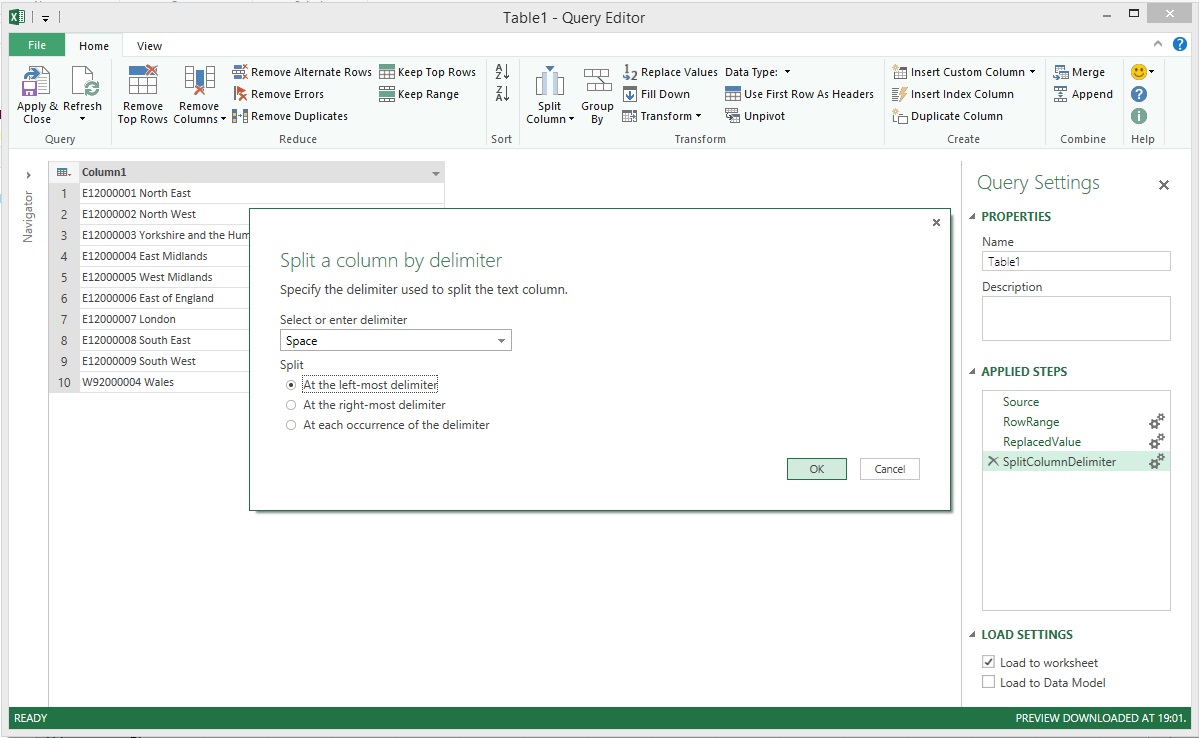
This is where the Split Column transformation came in handy. You will notice in the image above that in each row, the ID and name values are separated by a single blank space. This is why 'Space' was chosen for the Select or enter delimiter field and 'At the left-most delimiter' was chosen for the Split option. This told Power Query to look for the first blank space in each row and then use this to split the column.
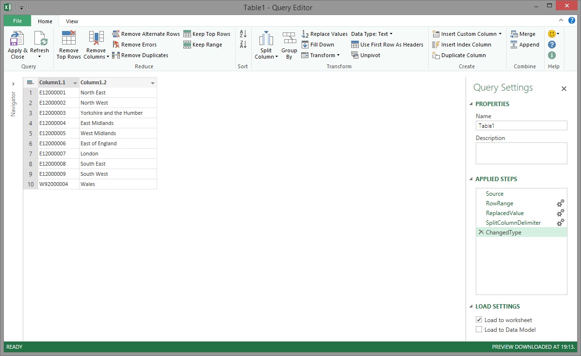
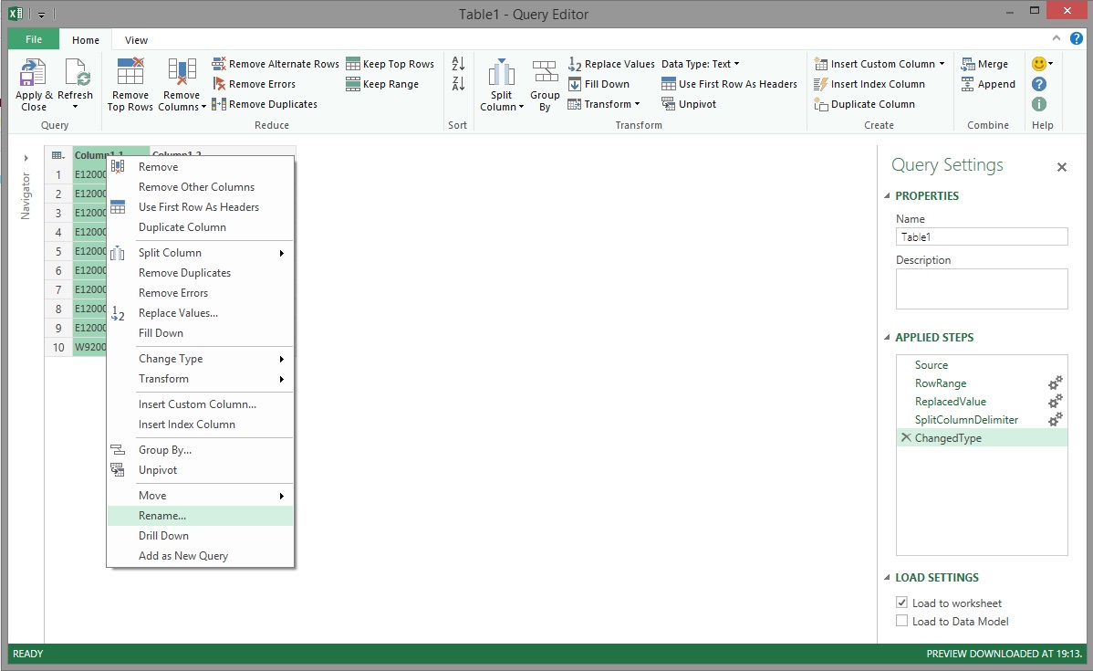
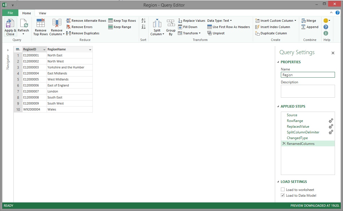
You can see in the image above that the values have been split into two columns and the table looks a lot more like the reference table that it was meant to be. The default columns names weren't meaningful so the the Rename transformation was used to give each a suitable name.
After renaming the columns, the Region table was finally in a good enough state to be loaded into Power Pivot. The query name was changed from 'Table1' to 'Region' and Power Query was told to only Load to Data Model before Apply & Close was clicked.
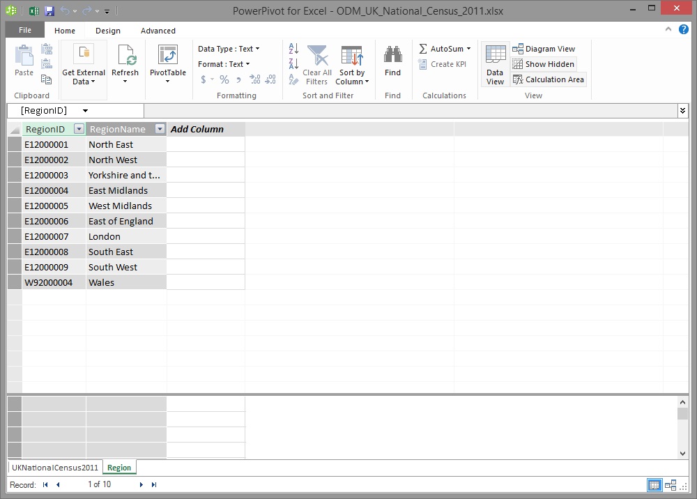
Within seconds, the 10 rows were successfully loaded into Power Pivot.
Let's take a quick look at the new Region table in the Power Pivot window's Data View...
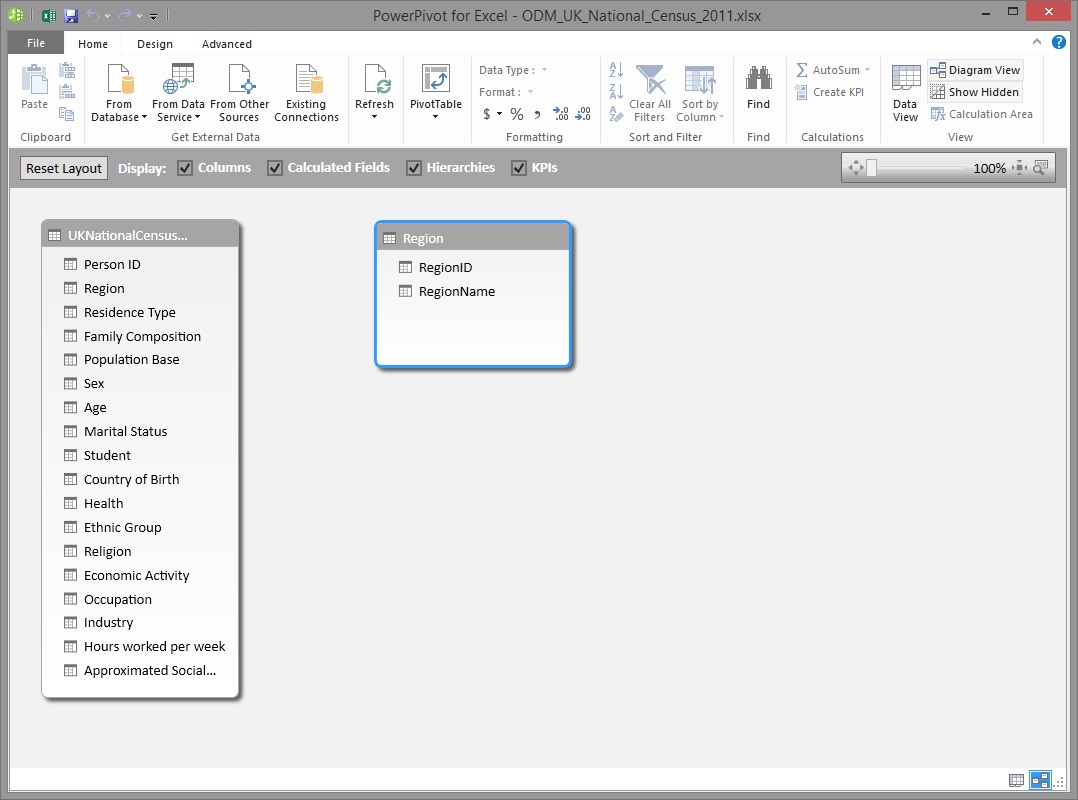
...And in the Power Pivot window's Diagram View...
Conclusion
As you've seen in the example presented by this article, Power Query makes it quick and relatively easy to get data into a good shape that can be loaded into Power Pivot to be modeled. Even though Power Query is quite a new tool, it already includes many of the common transformations that are required to handle both structured and unstructured data. In addition to this, it can be used to quickly prototype ETL logic that can later be used to support SSIS package ETL design and build activities.
Download the completed workbook
You can download the workbook from the TechNet Gallery.
Note: This article was adapted from this original blog post which also presents the completed Power Pivot Data Model and Power View data visualizations.