SDK 및 CLI를 사용하여 시계열 예측 모델을 학습하도록 AutoML을 설정합니다.
적용 대상: Azure CLI ml 확장 v2(현재)Python SDK azure-ai-ml v2(현재)
이 문서에서는 Azure Machine Learning Python SDK에서 Azure Machine Learning 자동화된 ML을 사용하여 시계열 예측을 위한 AutoML을 설정하는 방법을 알아봅니다.
이렇게 하려면 다음을 수행합니다.
- 학습을 위한 데이터를 준비합니다.
- 예측 작업에서 특정 시계열 매개 변수를 구성합니다.
- 구성 요소와 파이프라인을 사용하여 학습, 유추, 모델 평가를 조정합니다.
하위 코드 환경의 경우 Azure Machine Learning Studio에서 자동화된 ML을 사용하는 시계열 예측 예제를 알아보려면 자습서: 자동화된 Machine Learning으로 수요 예측을 참조하세요.
AutoML은 잘 알려진 시계열 모델과 함께 표준 기계 학습 모델을 사용하여 예측을 만듭니다. Microsoft의 방식은 대상 변수에 대한 기록 정보, 입력 데이터의 사용자 제공 기능 및 자동으로 엔지니어링된 기능을 통합합니다. 그러면 모델 검색 알고리즘이 작동하여 예측 정확도가 가장 높은 모델을 찾습니다. 자세한 내용은 예측 방법론 및 모델 검색에 대한 문서를 참조하세요.
필수 조건
이 문서의 내용을 진행하려면 다음 항목이 필요합니다.
Azure Machine Learning 작업 영역 작업 영역을 만들려면 작업 영역 리소스 만들기를 참조하세요.
AutoML 학습 작업을 시작하는 기능. 자세한 내용은 AutoML 설정 방법 가이드를 따릅니다.
학습 및 유효성 검사 데이터
AutoML 예측을 위한 입력 데이터는 테이블 형식의 유효한 시계열을 포함해야 합니다. 각 변수는 데이터 테이블에 고유한 해당 열이 있어야 합니다. AutoML에는 최소 두 개의 열이 필요합니다. 하나는 시간 축을 나타내는 시간 열이고 다른 하나는 예측할 수량인 대상 열입니다. 다른 열은 예측 변수 역할을 할 수 있습니다. 자세한 내용은 AutoML이 데이터를 사용하는 방법을 참조하세요.
Important
미래 가치를 예측하기 위해 모델을 학습하는 경우 학습에 사용된 모든 기능을 의도한 구간에 대해 예측을 실행할 때도 사용할 수 있는지 확인합니다.
예를 들어, 현재 주가에 대한 기능은 학습 정확도를 크게 높일 수 있습니다. 그러나 장기 구간을 사용하여 예측하려는 경우 미래 시계열 요소에 해당하는 선물 주가를 정확하게 예측할 수 없으며 모델 정확성이 떨어질 수 있습니다.
AutoML 예측 작업에서는 학습 데이터가 MLTable 개체로 표현되어야 합니다. MLTable은 데이터 원본 및 데이터 로드 단계를 지정합니다. 자세한 내용 및 사용 사례는 MLTable 방법 가이드를 참조하세요. 간단한 예로 학습 데이터가 로컬 디렉터리 ./train_data/timeseries_train.csv의 CSV 파일에 포함되어 있다고 가정합니다.
다음 예와 같이 mltable Python SDK를 사용하여 MLTable을 만들 수 있습니다.
import mltable

paths = [
    {'file': './train_data/timeseries_train.csv'}
]

train_table = mltable.from_delimited_files(paths)
train_table.save('./train_data')
이 코드는 파일 형식과 로드 지침이 포함된 새 파일 ./train_data/MLTable을 만듭니다.
이제 다음과 같이 Azure Machine Learning Python SDK를 사용하여 학습 작업을 시작하는 데 필요한 입력 데이터 개체를 정의합니다.
from azure.ai.ml.constants import AssetTypes
from azure.ai.ml import Input

# Training MLTable defined locally, with local data to be uploaded
my_training_data_input = Input(
    type=AssetTypes.MLTABLE, path="./train_data"
)
비슷한 방식으로 MLTable을 만들고 유효성 검사 데이터 입력을 지정하여 유효성 검사 데이터를 지정합니다. 또는 유효성 검사 데이터를 제공하지 않으면 AutoML은 모델 선택에 사용할 학습 데이터에서 교차 유효성 검사 분할을 자동으로 만듭니다. 자세한 내용은 예측 모델 선택에 대한 문서를 참조하세요. 또한 예측 모델을 성공적으로 학습시키는 데 필요한 학습 데이터의 양에 대한 자세한 내용은 학습 데이터 길이 요구 사항을 참조하세요.
AutoML이 교차 유효성 검사를 적용하여 과도 맞춤 방지하는 방법에 대해 자세히 알아봅니다.
실험 실행 컴퓨팅
AutoML은 완전 관리형 컴퓨팅 리소스인 Azure Machine Learning 컴퓨팅을 사용하여 학습 작업을 실행합니다. 다음 예에서는 cpu-compute라는 컴퓨팅 클러스터가 만들어집니다.
from azure.ai.ml.entities import AmlCompute

# specify aml compute name.
cpu_compute_target = "cpu-cluster"

try:
    ml_client.compute.get(cpu_compute_target)
except Exception:
    print("Creating a new cpu compute target...")
    compute = AmlCompute(
        name=cpu_compute_target, size="STANDARD_D2_V2", min_instances=0, max_instances=4
    )
ml_client.compute.begin_create_or_update(compute).result()실험 구성
automl 팩터리 함수를 사용하여 Python SDK에서 예측 작업을 구성합니다. 다음 예에서는 기본 메트릭을 설정하고 학습 실행에 대한 제한을 설정하여 예측 작업을 만드는 방법을 보여 줍니다.
from azure.ai.ml import automl

# note that the below is a code snippet -- you might have to modify the variable values to run it successfully
forecasting_job = automl.forecasting(
    compute="cpu-compute",
    experiment_name="sdk-v2-automl-forecasting-job",
    training_data=my_training_data_input,
    target_column_name=target_column_name,
    primary_metric="normalized_root_mean_squared_error",
    n_cross_validations="auto",
)

# Limits are all optional
forecasting_job.set_limits(
    timeout_minutes=120,
    trial_timeout_minutes=30,
    max_concurrent_trials=4,
)
예측 작업 설정
예측 작업에는 예측과 관련된 많은 설정이 있습니다. 이러한 설정 중 가장 기본적인 것은 학습 데이터의 시간 열 이름과 예측 범위입니다.
다음 설정을 구성하려면 ForecastingJob 메서드를 사용합니다.
# Forecasting specific configuration
forecasting_job.set_forecast_settings(
    time_column_name=time_column_name,
    forecast_horizon=24
)
시간 열 이름은 필수 설정이며 일반적으로 예측 시나리오에 따라 예측 범위를 설정해야 합니다. 데이터에 여러 시계열이 포함된 경우 시계열 ID 열의 이름을 지정할 수 있습니다. 이러한 열은 그룹화될 때 개별 계열을 정의합니다. 예를 들어, 다양한 저장소와 브랜드의 시간당 매출로 구성된 데이터가 있다고 가정합니다. 다음 샘플은 데이터에 "store" 및 "brand"라는 열이 포함되어 있다고 가정하고 시계열 ID 열을 설정하는 방법을 보여 줍니다.
# Forecasting specific configuration
# Add time series IDs for store and brand
forecasting_job.set_forecast_settings(
    ...,  # other settings
    time_series_id_column_names=['store', 'brand']
)
AutoML은 아무 것도 지정되지 않은 경우 데이터에서 시계열 ID 열을 자동으로 검색하려고 시도합니다.
다른 설정은 선택 사항이며 다음 섹션에서 검토됩니다.
선택적 예측 작업 설정
딥 러닝을 사용하도록 설정하고 대상 롤링 기간 집계를 지정하는 등의 예측 작업에 대한 옵션 구성을 사용할 수 있습니다. 전체 매개 변수 목록은 예측 참조 설명서 설명서에서 확인할 수 있습니다.
모델 검색 설정
AutoML이 최상의 모델인 allowed_training_algorithms 및 blocked_training_algorithms를 검색하는 모델 공간을 제어하는 두 가지 선택적 설정이 있습니다. 검색 공간을 특정 모델 클래스 집합으로 제한하려면 다음 샘플과 같이 allowed_training_algorithms 매개 변수를 사용합니다.
# Only search ExponentialSmoothing and ElasticNet models
forecasting_job.set_training(
    allowed_training_algorithms=["ExponentialSmoothing", "ElasticNet"]
)
이 경우 예측 작업은 지수 평활법 및 Elastic Net 모델 클래스만 검색합니다. 검색 공간에서 지정된 모델 클래스 집합을 제거하려면 다음 샘플과 같이 blocking_training_algorithms를 사용합니다.
# Search over all model classes except Prophet
forecasting_job.set_training(
    blocked_training_algorithms=["Prophet"]
)
이제 작업은 Prophet을 제외한 모든 모델 클래스를 검색합니다. allowed_training_algorithms 및 blocked_training_algorithms에서 허용되는 예측 모델 이름 목록은 학습 속성 참조 설명서를 확인합니다. allowed_training_algorithms와 blocked_training_algorithms 중 하나만 학습 실행에 적용할 수 있습니다.
딥 러닝 사용
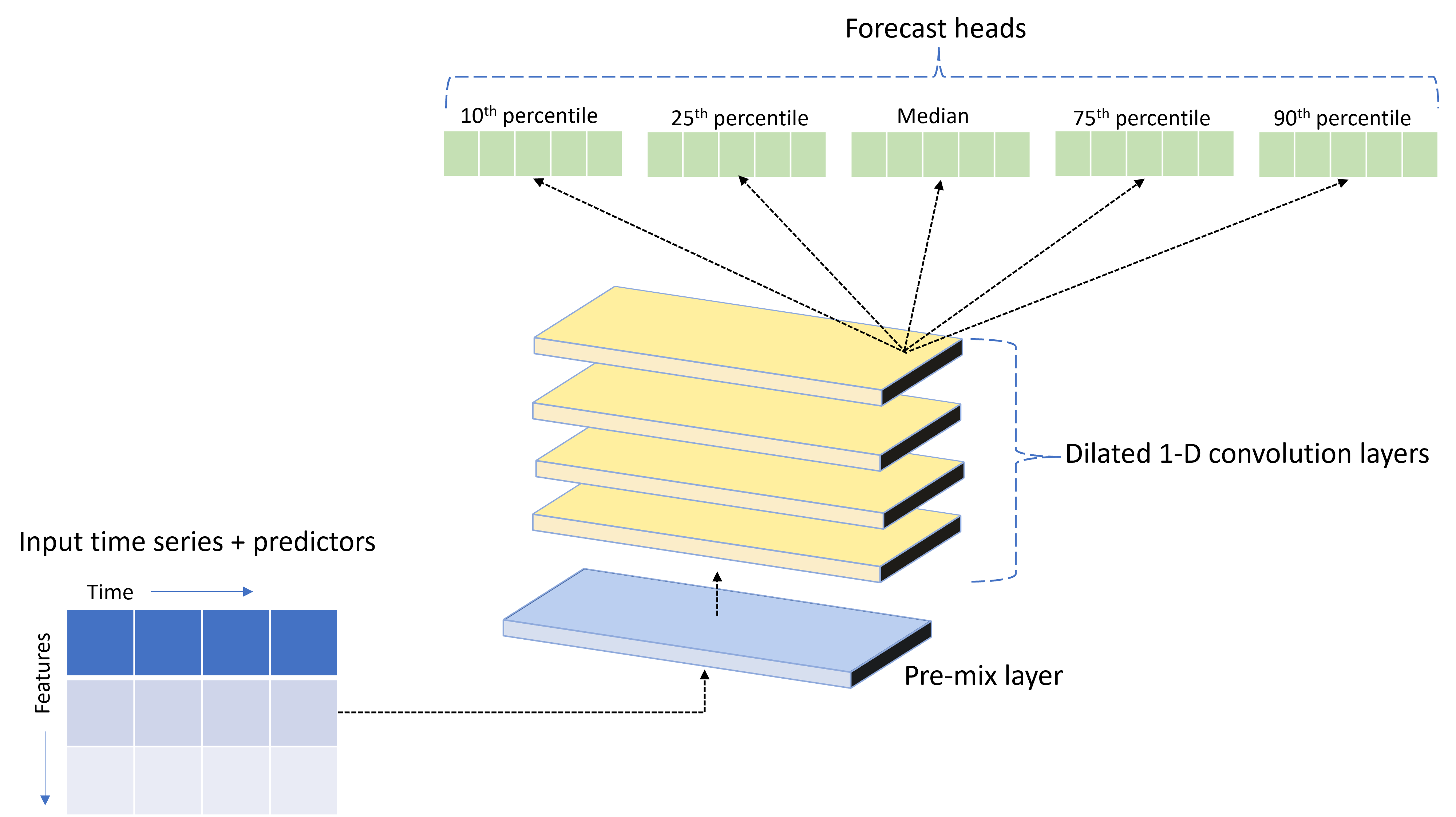
AutoML은 TCNForecaster라는 사용자 지정 DNN(심층 신경망) 모델과 함께 제공됩니다. 이 모델은 일반적인 이미징 작업 방법을 시계열 모델링에 적용하는 temporal convolutional network 또는 TCN입니다. 즉, 1차원 "인과 관계" 나선형은 네트워크의 중추를 형성하고 모델이 학습 기록에서 오랜 기간 동안 복잡한 패턴을 학습할 수 있도록 합니다. 자세한 내용은 TCNForecaster 문서를 참조하세요.
TCNForecaster는 학습 기록에 수천 개 이상의 관찰이 있는 경우 표준 시계열 모델보다 더 높은 정확도를 달성하는 경우가 많습니다. 그러나 용량이 더 크기 때문에 TCNForecaster 모델을 학습하고 스윕하는 데 시간이 더 걸립니다.
다음과 같이 학습 구성에서 enable_dnn_training 플래그를 설정하여 AutoML에서 TCNForecaster를 사용하도록 설정할 수 있습니다.
# Include TCNForecaster models in the model search
forecasting_job.set_training(
    enable_dnn_training=True
)
기본적으로 TCNForecaster 학습은 모델 시험당 단일 컴퓨팅 노드와 단일 GPU(사용 가능한 경우)로 제한됩니다. 대규모 데이터 시나리오의 경우 각 TCNForecaster 평가판을 여러 코어/GPU 및 노드에 배포하는 것이 좋습니다. 자세한 내용과 코드 샘플은 분산 학습 문서 섹션을 참조하세요.
Azure Machine Learning 스튜디오에서 만든 AutoML 실험에 DNN을 사용하도록 설정하려면 스튜디오 UI에서 작업 유형 설정 방법을 참조하세요.
참고 항목
- SDK로 만든 실험에 DNN을 사용하도록 설정하면 최상의 모델 설명이 사용하지 않도록 설정됩니다.
- 자동화된 Machine Learning의 예측에 대한 DNN 지원은 Databricks에서 시작된 실행에 대해 지원되지 않습니다.
- DNN 학습이 사용하도록 설정된 경우 GPU 컴퓨팅 형식이 권장됩니다.
지연 및 롤링 창 기능
대상의 최근 값은 종종 예측 모델에서 영향력 있는 기능입니다. 따라서 AutoML은 시간 지연 및 롤링 창 집계 기능을 만들어 잠재적으로 모델 정확도를 개선시킬 수 있습니다.
날씨 데이터와 과거 수요를 사용할 수 있는 에너지 수요 예측 시나리오를 고려합니다. 표는 가장 최근 3시간 동안 기간 집계가 적용될 때 발생하는 결과 기능 엔지니어링을 보여 줍니다. 최소, 최대 및 합계 열은 정의된 설정을 기반으로 3시간 슬라이딩 윈도우에서 생성됩니다. 예를 들어, 2017년 9월 8일 오전 4시에 유효한 관찰의 경우 최댓값, 최솟값 및 합계 값은 2017년 9월 8일 오전 1시 - 오전 3시에 대한 수요 값을 사용하여 계산됩니다. 이 3시간의 기간은 나머지 행에 대한 데이터를 채우기 위해 이동합니다. 자세한 내용과 예를 보려면 지연 기능 문서을 참조하세요.

롤링 창 크기(이전 예에서는 3개)와 만들려는 지연 순서를 설정하여 대상에 대한 지연 및 롤링 창 집계 기능을 사용하도록 설정할 수 있습니다. feature_lags 설정을 사용하여 기능에 대한 지연을 사용하도록 설정할 수도 있습니다. 다음 샘플에서는 AutoML이 데이터의 상관 구조를 분석하여 자동으로 설정을 결정할 수 있도록 이러한 설정을 모두 auto로 설정했습니다.
forecasting_job.set_forecast_settings(
    ...,  # other settings
    target_lags='auto',
    target_rolling_window_size='auto',
    feature_lags='auto'
)
짧은 계열 처리
자동화된 ML은 모델 개발의 학습 및 유효성 검사 단계를 수행하기에 충분한 데이터 요소가 없으면 시계열을 짧은 계열로 간주합니다. 길이 요구 사항에 대한 자세한 내용은 학습 데이터 길이 요구 사항을 참조하세요.
AutoML에는 짧은 시리즈에 대해 수행할 수 있는 몇 가지 작업이 있습니다. 이러한 작업은 short_series_handling_config 설정으로 구성할 수 있습니다. 기본값은 "자동"입니다. 다음 표에서는 설정에 대해 설명합니다.
| 설정 | 설명 |
|---|---|
auto |
짧은 계열 처리의 기본값입니다. - 모든 계열이 짧은 경우 데이터를 패딩합니다. - 모든 계열이 짧은 것은 아닌 경우 짧은 계열을 삭제합니다. |
pad |
short_series_handling_config = pad인 경우 자동화된 ML은 찾아낸 각 짧은 계열에 임의 값을 추가합니다. 다음 목록에는 열 유형과 채워지는 항목이 나와 있습니다. - NaN으로 채워지는 개체 열 - 0으로 채워지는 숫자 열 - False로 채워지는 부울/논리 열 - 대상 열은 백색 소음으로 채워집니다. |
drop |
short_series_handling_config = drop인 경우 자동화된 ML이 짧은 계열을 삭제하여 학습 또는 예측에 사용되지 않습니다. 이러한 계열에 대한 예측은 NaN을 반환합니다. |
None |
채워지거나 삭제된 계열이 없음 |
다음 예에서는 모든 짧은 시리즈가 최소 길이로 채워지도록 짧은 시리즈 처리를 설정합니다.
forecasting_job.set_forecast_settings(
    ...,  # other settings
    short_series_handling_config='pad'
)
Warning
학습 실패를 방지하기 위해 인공 데이터를 도입하므로 패딩은 결과 모델의 정확도에 영향을 미칠 수 있습니다. 많은 계열이 짧은 경우 설명 가능성 결과에 어느 정도 영향이 있을 수 있습니다.
빈도 및 대상 데이터 집계
빈도 및 데이터 집계 옵션을 사용하여 불규칙한 데이터로 인한 장애를 방지합니다. 데이터가 시간별 또는 일별과 같이 정해진 주기를 따르지 않으면 데이터가 불규칙합니다. POS 데이터는 비정형 데이터의 좋은 예입니다. 이러한 경우 AutoML은 데이터를 원하는 빈도로 집계한 다음 집계에서 예측 모델을 빌드할 수 있습니다.
불규칙한 데이터를 처리하려면 frequency 및 target_aggregate_function 설정을 지정해야 합니다. 빈도 설정은 Pandas DateOffset 문자열을 입력으로 허용합니다. 집계 함수에 대해 지원되는 값은 다음과 같습니다.
| 함수 | 설명 |
|---|---|
sum |
대상 값의 합계 |
mean |
대상 값의 평균 또는 산술평균 |
min |
대상의 최솟값 |
max |
대상의 최댓값 |
- 지정된 작업에 따라 대상 열 값이 집계됩니다. 일반적으로 sum은 대부분의 시나리오에 적합합니다.
- 데이터의 숫자 예측 요소 열은 합계, 평균, 최솟값 및 최댓값으로 집계됩니다. 결과적으로 자동화된 ML은 집계 함수 이름이 접미사인 새 열을 생성하고 선택된 집계 작업을 적용합니다.
- 범주 예측요소 열의 경우 데이터는 기간 내에 가장 두드러진 범주인 최빈값으로 집계됩니다.
- 날짜 예측 열은 최솟값, 최댓값 및 최빈값으로 집계됩니다.
다음 예에서는 빈도를 매시간으로 설정하고 집계 함수를 합계로 설정합니다.
# Aggregate the data to hourly frequency
forecasting_job.set_forecast_settings(
    ...,  # other settings
    frequency='H',
    target_aggregate_function='sum'
)
사용자 지정 교차 유효성 검사 설정
예측 작업에 대한 교차 유효성 검사를 제어하는 두 가지 사용자 지정 가능한 설정, 즉 접기 수, n_cross_validations및 접기 간의 시간 오프셋을 정의하는 단계 크기 cv_step_size가 있습니다. 이러한 매개 변수의 의미에 대한 자세한 내용은 예측 모델 선택을 참조하세요. 기본적으로 AutoML은 데이터의 특성을 기반으로 두 설정을 자동으로 설정하지만 고급 사용자는 수동으로 설정할 수 있습니다. 예를 들어, 일별 판매 데이터가 있고 인접한 접기 사이에 7일 오프셋이 있는 다섯 개의 접기로 유효성 검사 설정을 구성하려고 한다고 가정합니다. 다음 코드 샘플은 이를 설정하는 방법을 보여 줍니다.
from azure.ai.ml import automl

# Create a job with five CV folds
forecasting_job = automl.forecasting(
    ...,  # other training parameters
    n_cross_validations=5,
)

# Set the step size between folds to seven days
forecasting_job.set_forecast_settings(
    ...,  # other settings
    cv_step_size=7
)
사용자 지정 기능화
기본적으로 AutoML은 엔지니어링된 기능으로 학습 데이터를 보강하여 모델의 정확도를 높입니다. 자세한 내용은 자동 기능 엔지니어링을 참조하세요. 일부 전처리 단계는 예측 작업의 기능화 구성을 사용하여 사용자 지정할 수 있습니다.
예측에 지원되는 사용자 지정은 다음 표에 나와 있습니다.
| 사용자 지정 | 설명 | Options |
|---|---|---|
| 열 용도 업데이트 | 지정된 열에 대해 자동 감지된 기능 유형을 재정의합니다. | "Categorical", "DateTime", "Numeric" |
| 변환기 매개 변수 업데이트 | 지정된 imputer의 매개 변수를 업데이트합니다. | {"strategy": "constant", "fill_value": <value>}, {"strategy": "median"}, {"strategy": "ffill"} |
예를 들어, 데이터에 가격, "세일 중" 플래그 및 제품 형식이 포함된 소매 수요 시나리오가 있다고 가정합니다. 다음 샘플은 이러한 기능에 대한 사용자 지정 형식 및 imputer를 설정하는 방법을 보여 줍니다.
from azure.ai.ml.automl import ColumnTransformer

# Customize imputation methods for price and is_on_sale features
# Median value imputation for price, constant value of zero for is_on_sale
transformer_params = {
    "imputer": [
        ColumnTransformer(fields=["price"], parameters={"strategy": "median"}),
        ColumnTransformer(fields=["is_on_sale"], parameters={"strategy": "constant", "fill_value": 0}),
    ],
}

# Set the featurization
# Ensure that product_type feature is interpreted as categorical
forecasting_job.set_featurization(
    mode="custom",
    transformer_params=transformer_params,
    column_name_and_types={"product_type": "Categorical"},
)
실험에 Azure Machine Learning 스튜디오를 사용하는 경우 스튜디오에서 기능화를 사용자 지정하는 방법을 참조하세요.
예측 작업 제출
모든 설정을 구성한 후 다음과 같이 예측 작업을 시작합니다.
# Submit the AutoML job
returned_job = ml_client.jobs.create_or_update(
    forecasting_job
)

print(f"Created job: {returned_job}")

# Get a URL for the job in the AML studio user interface
returned_job.services["Studio"].endpoint
작업이 제출되면 AutoML은 컴퓨팅 리소스를 프로비전하고 입력 데이터에 기능화 및 기타 준비 단계를 적용한 다음 예측 모델을 전면적으로 조사하기 시작합니다. 자세한 내용은 예측 방법론 및 모델 검색에 대한 문서를 참조하세요.
구성 요소 및 파이프라인을 사용하여 학습, 유추, 평가 오케스트레이션
Important
이 기능은 현재 공개 미리 보기로 제공됩니다. 이 미리 보기 버전은 서비스 수준 계약 없이 제공되며, 프로덕션 워크로드에는 권장되지 않습니다. 특정 기능이 지원되지 않거나 기능이 제한될 수 있습니다.
자세한 내용은 Microsoft Azure Preview에 대한 추가 사용 약관을 참조하세요.
ML 워크플로에는 단순한 학습 이상의 것이 필요할 수 있습니다. 유추, 최신 데이터에 대한 모델 예측 검색, 알려진 대상 값이 있는 테스트 집합의 모델 정확도 평가는 학습 작업과 함께 AzureML에서 오케스트레이션할 수 있는 다른 일반적인 작업입니다. 유추 및 평가 작업을 지원하기 위해 AzureML은 AzureML 파이프라인에서 한 단계를 수행하는 독립형 코드 조각인 구성 요소를 제공합니다.
다음 예에서는 클라이언트 레지스트리에서 구성 요소 코드를 검색합니다.
from azure.ai.ml import MLClient
from azure.identity import DefaultAzureCredential, InteractiveBrowserCredential

# Get a credential for access to the AzureML registry
try:
    credential = DefaultAzureCredential()
    # Check if we can get token successfully.
    credential.get_token("https://management.azure.com/.default")
except Exception as ex:
    # Fall back to InteractiveBrowserCredential in case DefaultAzureCredential fails
    credential = InteractiveBrowserCredential()

# Create a client for accessing assets in the AzureML preview registry
ml_client_registry = MLClient(
    credential=credential,
    registry_name="azureml-preview"
)

# Create a client for accessing assets in the AzureML preview registry
ml_client_metrics_registry = MLClient(
    credential=credential,
    registry_name="azureml"
)

# Get an inference component from the registry
inference_component = ml_client_registry.components.get(
    name="automl_forecasting_inference",
    label="latest"
)

# Get a component for computing evaluation metrics from the registry
compute_metrics_component = ml_client_metrics_registry.components.get(
    name="compute_metrics",
    label="latest"
)
다음으로 학습, 유추, 메트릭 계산을 오케스트레이션하는 파이프라인을 만드는 팩터리 함수를 정의합니다. 학습 설정에 대한 자세한 내용은 학습 구성 섹션을 참조하세요.
from azure.ai.ml import automl
from azure.ai.ml.constants import AssetTypes
from azure.ai.ml.dsl import pipeline

@pipeline(description="AutoML Forecasting Pipeline")
def forecasting_train_and_evaluate_factory(
    train_data_input,
    test_data_input,
    target_column_name,
    time_column_name,
    forecast_horizon,
    primary_metric='normalized_root_mean_squared_error',
    cv_folds='auto'
):
    # Configure the training node of the pipeline
    training_node = automl.forecasting(
        training_data=train_data_input,
        target_column_name=target_column_name,
        primary_metric=primary_metric,
        n_cross_validations=cv_folds,
        outputs={"best_model": Output(type=AssetTypes.MLFLOW_MODEL)},
    )

    training_node.set_forecasting_settings(
        time_column_name=time_column_name,
        forecast_horizon=max_horizon,
        frequency=frequency,
        # other settings
        ...
    )

    training_node.set_training(
        # training parameters
        ...
    )

    training_node.set_limits(
        # limit settings
        ...
    )

    # Configure the inference node to make rolling forecasts on the test set
    inference_node = inference_component(
        test_data=test_data_input,
        model_path=training_node.outputs.best_model,
        target_column_name=target_column_name,
        forecast_mode='rolling',
        forecast_step=1
    )

    # Configure the metrics calculation node
    compute_metrics_node = compute_metrics_component(
        task="tabular-forecasting",
        ground_truth=inference_node.outputs.inference_output_file,
        prediction=inference_node.outputs.inference_output_file,
        evaluation_config=inference_node.outputs.evaluation_config_output_file
    )

    # return a dictionary with the evaluation metrics and the raw test set forecasts
    return {
        "metrics_result": compute_metrics_node.outputs.evaluation_result,
        "rolling_fcst_result": inference_node.outputs.inference_output_file
    }
이제 로컬 폴더 ./train_data 및 ./test_data에 포함되어 있다고 가정하여 학습 및 테스트 데이터 입력을 정의합니다.
my_train_data_input = Input(
    type=AssetTypes.MLTABLE,
    path="./train_data"
)

my_test_data_input = Input(
    type=AssetTypes.URI_FOLDER,
    path='./test_data',
)
마지막으로 파이프라인을 구성하고 기본 컴퓨팅을 설정한 후 작업을 제출합니다.
pipeline_job = forecasting_train_and_evaluate_factory(
    my_train_data_input,
    my_test_data_input,
    target_column_name,
    time_column_name,
    forecast_horizon
)

# set pipeline level compute
pipeline_job.settings.default_compute = compute_name

# submit the pipeline job
returned_pipeline_job = ml_client.jobs.create_or_update(
    pipeline_job,
    experiment_name=experiment_name
)
returned_pipeline_job
제출되면 파이프라인은 AutoML 학습, 롤링 평가 유추, 메트릭 계산을 순서대로 실행합니다. 스튜디오 UI에서 실행을 모니터링하고 검사할 수 있습니다. 실행이 완료되면 롤링 예측과 평가 메트릭을 로컬 작업 디렉터리에 다운로드할 수 있습니다.
# Download the metrics json
ml_client.jobs.download(returned_pipeline_job.name, download_path=".", output_name='metrics_result')

# Download the rolling forecasts
ml_client.jobs.download(returned_pipeline_job.name, download_path=".", output_name='rolling_fcst_result')
그런 다음 ./named-outputs/metrics_results/evaluationResult/metrics.json에서 메트릭 결과를 찾을 수 있고 ./named-outputs/rolling_fcst_result/inference_output_file에서 JSON 라인 형식의 예측을 찾을 수 있습니다.
롤링 평가에 대한 자세한 내용은 예측 모델 평가 문서를 참조하세요.
대규모 예측: 다양한 모델
Important
이 기능은 현재 공개 미리 보기로 제공됩니다. 이 미리 보기 버전은 서비스 수준 계약 없이 제공되며, 프로덕션 워크로드에는 권장되지 않습니다. 특정 기능이 지원되지 않거나 기능이 제한될 수 있습니다.
자세한 내용은 Microsoft Azure Preview에 대한 추가 사용 약관을 참조하세요.
AutoML의 다양한 모델 구성 요소를 사용하면 수백만 개의 모델을 동시에 학습하고 관리할 수 있습니다. 다양한 모델 개념에 대한 자세한 내용은 다양한 모델 문서 섹션을 참조하세요.
많은 모델 학습 구성
다중 모델 학습 구성 요소는 AutoML 학습 설정의 YAML 형식 구성 파일을 허용합니다. 구성 요소는 시작하는 각 AutoML 인스턴스에 이러한 설정을 적용합니다. 이 YAML 파일에는 예측 작업과 동일한 사양과 추가 매개 변수 partition_column_names 및 allow_multi_partitions가 있습니다.
| 매개 변수 | 설명 |
|---|---|
| partition_column_names | 그룹화될 때 데이터 파티션을 정의하는 데이터의 열 이름입니다. 다중 모델 학습 구성 요소는 각 파티션에서 독립적인 학습 작업을 시작합니다. |
| allow_multi_partitions | 각 파티션에 둘 이상의 고유한 시계열이 포함된 경우 파티션당 하나의 모델을 학습할 수 있는 선택적 플래그입니다. 기본값은 False입니다. |
다음 샘플은 구성 템플릿을 제공합니다.
$schema: https://azuremlsdk2.blob.core.windows.net/preview/0.0.1/autoMLJob.schema.json
type: automl

description: A time series forecasting job config
compute: azureml:<cluster-name>
task: forecasting
primary_metric: normalized_root_mean_squared_error
target_column_name: sales
n_cross_validations: 3

forecasting:
  time_column_name: date
  time_series_id_column_names: ["state", "store"]
  forecast_horizon: 28

training:
  blocked_training_algorithms: ["ExtremeRandomTrees"]

limits:
  timeout_minutes: 15
  max_trials: 10
  max_concurrent_trials: 4
  max_cores_per_trial: -1
  trial_timeout_minutes: 15
  enable_early_termination: true

partition_column_names: ["state", "store"]
allow_multi_partitions: false
후속 예에서는 구성이 ./automl_settings_mm.yml 경로에 저장되어 있다고 가정합니다.
많은 모델 파이프라인
다음으로, 많은 모델 학습, 유추, 메트릭 계산의 오케스트레이션을 위한 파이프라인을 만드는 팩터리 함수를 정의합니다. 이 팩터리 함수의 매개 변수는 다음 표에 자세히 설명되어 있습니다.
| 매개 변수 | 설명 |
|---|---|
| max_nodes | 학습 작업에 사용할 컴퓨팅 노드 수 |
| max_concurrency_per_node | 각 노드에서 실행할 AutoML 프로세스 수입니다. 따라서 많은 모델 작업의 총 동시성은 max_nodes * max_concurrency_per_node입니다. |
| parallel_step_timeout_in_seconds | 많은 모델 구성 요소 시간 제한이 초 단위로 제공됩니다. |
| retrain_failed_models | 실패한 모델에 대한 재학습을 사용하도록 설정하는 플래그입니다. 이는 이전에 일부 데이터 파티션에서 AutoML 작업이 실패한 여러 모델 실행을 수행한 경우에 유용합니다. 이 플래그가 사용하도록 설정되면 많은 모델은 이전에 실패한 파티션에 대해서만 학습 작업을 시작합니다. |
| forecast_mode | 모델 평가를 위한 유추 모드입니다. 유효한 값은 "recursive" 및 "rolling"입니다. 자세한 내용은 모델 평가 문서를 참조하세요. |
| forecast_step | 롤링 예측의 단계 크기입니다. 자세한 내용은 모델 평가 문서를 참조하세요. |
다음 샘플은 많은 모델 학습 및 모델 평가 파이프라인을 구성하기 위한 팩터리 방법을 보여 줍니다.
from azure.ai.ml import MLClient
from azure.identity import DefaultAzureCredential, InteractiveBrowserCredential

# Get a credential for access to the AzureML registry
try:
    credential = DefaultAzureCredential()
    # Check if we can get token successfully.
    credential.get_token("https://management.azure.com/.default")
except Exception as ex:
    # Fall back to InteractiveBrowserCredential in case DefaultAzureCredential fails
    credential = InteractiveBrowserCredential()

# Get a many models training component
mm_train_component = ml_client_registry.components.get(
    name='automl_many_models_training',
    version='latest'
)

# Get a many models inference component
mm_inference_component = ml_client_registry.components.get(
    name='automl_many_models_inference',
    version='latest'
)

# Get a component for computing evaluation metrics
compute_metrics_component = ml_client_metrics_registry.components.get(
    name="compute_metrics",
    label="latest"
)
@pipeline(description="AutoML Many Models Forecasting Pipeline")
def many_models_train_evaluate_factory(
    train_data_input,
    test_data_input,
    automl_config_input,
    compute_name,
    max_concurrency_per_node=4,
    parallel_step_timeout_in_seconds=3700,
    max_nodes=4,
    retrain_failed_model=False,
    forecast_mode="rolling",
    forecast_step=1
):
    mm_train_node = mm_train_component(
        raw_data=train_data_input,
        automl_config=automl_config_input,
        max_nodes=max_nodes,
        max_concurrency_per_node=max_concurrency_per_node,
        parallel_step_timeout_in_seconds=parallel_step_timeout_in_seconds,
        retrain_failed_model=retrain_failed_model,
        compute_name=compute_name
    )

    mm_inference_node = mm_inference_component(
        raw_data=test_data_input,
        max_nodes=max_nodes,
        max_concurrency_per_node=max_concurrency_per_node,
        parallel_step_timeout_in_seconds=parallel_step_timeout_in_seconds,
        optional_train_metadata=mm_train_node.outputs.run_output,
        forecast_mode=forecast_mode,
        forecast_step=forecast_step,
        compute_name=compute_name
    )

    compute_metrics_node = compute_metrics_component(
        task="tabular-forecasting",
        prediction=mm_inference_node.outputs.evaluation_data,
        ground_truth=mm_inference_node.outputs.evaluation_data,
        evaluation_config=mm_inference_node.outputs.evaluation_configs
    )

    # Return the metrics results from the rolling evaluation
    return {
        "metrics_result": compute_metrics_node.outputs.evaluation_result
    }
이제 학습 및 테스트 데이터가 각각 로컬 폴더 ./data/train 및 ./data/test에 있다고 가정하고 팩터리 함수를 통해 파이프라인을 구성합니다. 마지막으로 다음 샘플과 같이 기본 컴퓨팅을 설정하고 작업을 제출합니다.
pipeline_job = many_models_train_evaluate_factory(
    train_data_input=Input(
        type="uri_folder",
        path="./data/train"
    ),
    test_data_input=Input(
        type="uri_folder",
        path="./data/test"
    ),
    automl_config=Input(
        type="uri_file",
        path="./automl_settings_mm.yml"
    ),
    compute_name="<cluster name>"
)
pipeline_job.settings.default_compute = "<cluster name>"

returned_pipeline_job = ml_client.jobs.create_or_update(
    pipeline_job,
    experiment_name=experiment_name,
)
ml_client.jobs.stream(returned_pipeline_job.name)
작업이 완료된 후 단일 학습 실행 파이프라인과 동일한 절차를 사용하여 평가 메트릭을 로컬로 다운로드할 수 있습니다.
자세한 예는 다양한 모델을 사용한 수요 예측 Notebook을 참조하세요.
참고 항목
많은 모델 학습 및 유추 구성 요소는 각 파티션이 자체 파일에 있도록 partition_column_names 설정에 따라 조건부로 데이터를 분할합니다. 데이터가 매우 큰 경우 이 프로세스가 매우 느리거나 실패할 수 있습니다. 이 경우 많은 모델 학습 또는 유추를 실행하기 전에 데이터를 수동으로 분할하는 것이 좋습니다.
대규모 예측: 계층적 시계열
Important
이 기능은 현재 공개 미리 보기로 제공됩니다. 이 미리 보기 버전은 서비스 수준 계약 없이 제공되며, 프로덕션 워크로드에는 권장되지 않습니다. 특정 기능이 지원되지 않거나 기능이 제한될 수 있습니다.
자세한 내용은 Microsoft Azure Preview에 대한 추가 사용 약관을 참조하세요.
AutoML의 HTS(계층적 시계열) 구성 요소를 사용하면 계층 구조의 데이터에 대해 수많은 모델을 학습할 수 있습니다. 자세한 내용은 HTS 문서 섹션을 참조하세요.
HTS 학습 구성
HTS 학습 구성 요소는 AutoML 학습 설정의 YAML 형식 구성 파일을 허용합니다. 구성 요소는 시작하는 각 AutoML 인스턴스에 이러한 설정을 적용합니다. 이 YAML 파일에는 예측 작업과 동일한 사양과 계층 구조 정보와 관련된 추가 매개 변수가 있습니다.
| 매개 변수 | 설명 |
|---|---|
| hierarchy_column_names | 데이터의 계층 구조를 정의하는 데이터의 열 이름 목록입니다. 이 목록의 열 순서에 따라 계층 구조 수준이 결정됩니다. 목록 인덱스에 따라 집계 정도가 감소합니다. 즉, 목록의 마지막 열은 계층 구조의 리프(가장 세분화된) 수준을 정의합니다. |
| hierarchy_training_level | 예측 모델 학습에 사용할 계층 구조 수준입니다. |
다음은 샘플 구성을 보여 줍니다.
$schema: https://azuremlsdk2.blob.core.windows.net/preview/0.0.1/autoMLJob.schema.json
type: automl

description: A time series forecasting job config
compute: azureml:cluster-name
task: forecasting
primary_metric: normalized_root_mean_squared_error
log_verbosity: info
target_column_name: sales
n_cross_validations: 3

forecasting:
  time_column_name: "date"
  time_series_id_column_names: ["state", "store", "SKU"]
  forecast_horizon: 28

training:
  blocked_training_algorithms: ["ExtremeRandomTrees"]

limits:
  timeout_minutes: 15
  max_trials: 10
  max_concurrent_trials: 4
  max_cores_per_trial: -1
  trial_timeout_minutes: 15
  enable_early_termination: true

hierarchy_column_names: ["state", "store", "SKU"]
hierarchy_training_level: "store"
후속 예에서는 구성이 ./automl_settings_hts.yml 경로에 저장되어 있다고 가정합니다.
HTS 파이프라인
다음으로, HTS 학습, 유추, 메트릭 계산의 오케스트레이션을 위한 파이프라인을 만드는 팩터리 함수를 정의합니다. 이 팩터리 함수의 매개 변수는 다음 표에 자세히 설명되어 있습니다.
| 매개 변수 | 설명 |
|---|---|
| forecast_level | 예측을 검색할 계층 구조 수준 |
| allocation_method | 예측이 세분화될 때 사용할 할당 방법입니다. 유효한 값은 "proportions_of_historical_average" 및 "average_historical_proportions"입니다. |
| max_nodes | 학습 작업에 사용할 컴퓨팅 노드 수 |
| max_concurrency_per_node | 각 노드에서 실행할 AutoML 프로세스 수입니다. 따라서 HTS 작업의 총 동시성은 max_nodes * max_concurrency_per_node입니다. |
| parallel_step_timeout_in_seconds | 많은 모델 구성 요소 시간 제한이 초 단위로 제공됩니다. |
| forecast_mode | 모델 평가를 위한 유추 모드입니다. 유효한 값은 "recursive" 및 "rolling"입니다. 자세한 내용은 모델 평가 문서를 참조하세요. |
| forecast_step | 롤링 예측의 단계 크기입니다. 자세한 내용은 모델 평가 문서를 참조하세요. |
from azure.ai.ml import MLClient
from azure.identity import DefaultAzureCredential, InteractiveBrowserCredential

# Get a credential for access to the AzureML registry
try:
    credential = DefaultAzureCredential()
    # Check if we can get token successfully.
    credential.get_token("https://management.azure.com/.default")
except Exception as ex:
    # Fall back to InteractiveBrowserCredential in case DefaultAzureCredential fails
    credential = InteractiveBrowserCredential()

# Get a HTS training component
hts_train_component = ml_client_registry.components.get(
    name='automl_hts_training',
    version='latest'
)

# Get a HTS inference component
hts_inference_component = ml_client_registry.components.get(
    name='automl_hts_inference',
    version='latest'
)

# Get a component for computing evaluation metrics
compute_metrics_component = ml_client_metrics_registry.components.get(
    name="compute_metrics",
    label="latest"
)
@pipeline(description="AutoML HTS Forecasting Pipeline")
def hts_train_evaluate_factory(
    train_data_input,
    test_data_input,
    automl_config_input,
    max_concurrency_per_node=4,
    parallel_step_timeout_in_seconds=3700,
    max_nodes=4,
    forecast_mode="rolling",
    forecast_step=1,
    forecast_level="SKU",
    allocation_method='proportions_of_historical_average'
):
    hts_train = hts_train_component(
        raw_data=train_data_input,
        automl_config=automl_config_input,
        max_concurrency_per_node=max_concurrency_per_node,
        parallel_step_timeout_in_seconds=parallel_step_timeout_in_seconds,
        max_nodes=max_nodes
    )
    hts_inference = hts_inference_component(
        raw_data=test_data_input,
        max_nodes=max_nodes,
        max_concurrency_per_node=max_concurrency_per_node,
        parallel_step_timeout_in_seconds=parallel_step_timeout_in_seconds,
        optional_train_metadata=hts_train.outputs.run_output,
        forecast_level=forecast_level,
        allocation_method=allocation_method,
        forecast_mode=forecast_mode,
        forecast_step=forecast_step
    )
    compute_metrics_node = compute_metrics_component(
        task="tabular-forecasting",
        prediction=hts_inference.outputs.evaluation_data,
        ground_truth=hts_inference.outputs.evaluation_data,
        evaluation_config=hts_inference.outputs.evaluation_configs
    )

    # Return the metrics results from the rolling evaluation
    return {
        "metrics_result": compute_metrics_node.outputs.evaluation_result
    }
이제 학습 및 테스트 데이터가 각각 로컬 폴더 ./data/train 및 ./data/test에 있다고 가정하고 팩터리 함수를 통해 파이프라인을 구성합니다. 마지막으로 다음 샘플과 같이 기본 컴퓨팅을 설정하고 작업을 제출합니다.
pipeline_job = hts_train_evaluate_factory(
    train_data_input=Input(
        type="uri_folder",
        path="./data/train"
    ),
    test_data_input=Input(
        type="uri_folder",
        path="./data/test"
    ),
    automl_config=Input(
        type="uri_file",
        path="./automl_settings_hts.yml"
    )
)
pipeline_job.settings.default_compute = "cluster-name"

returned_pipeline_job = ml_client.jobs.create_or_update(
    pipeline_job,
    experiment_name=experiment_name,
)
ml_client.jobs.stream(returned_pipeline_job.name)
작업이 완료된 후 단일 학습 실행 파이프라인과 동일한 절차를 사용하여 평가 메트릭을 로컬로 다운로드할 수 있습니다.
자세한 예는 계층적 시계열 Notebook을 사용한 수요 예측을 참조하세요.
참고 항목
HTS 학습 및 유추 구성 요소는 각 파티션이 자체 파일에 있도록 hierarchy_column_names 설정에 따라 조건부로 데이터를 분할합니다. 데이터가 매우 큰 경우 이 프로세스가 매우 느리거나 실패할 수 있습니다. 이 경우 HTS 학습 또는 유추를 실행하기 전에 데이터를 수동으로 분할하는 것이 좋습니다.
대규모 예측: 분산 DNN 학습
- 예측 작업에 분산 학습이 어떻게 작동하는지 알아보려면 대규모 예측 문서를 참조하세요.
- 코드 샘플은 표 형식 데이터에 대한 분산 학습 설정 문서 섹션을 참조하세요.
예제 Notebook
다음을 포함하는 고급 예측 구성의 자세한 코드 예제는 예측 샘플 Notebook을 참조하세요.
다음 단계
- AutoML 모델을 온라인 엔드포인트에 배포하는 방법에 대해 자세히 알아봅니다.
- 해석력: 자동화된 Machine Learning의 모델 설명(미리 보기)에 대해 알아봅니다.
- AutoML이 예측 모델을 빌드하는 방법에 대해 알아봅니다.
- 대규모 예측에 대해 알아봅니다.
- 다양한 예측 시나리오에 맞게 AutoML을 구성하는 방법에 대해 알아봅니다.
- 예측 모델의 유추 및 평가에 대해 알아봅니다.