Python 해석력 패키지를 사용하여 ML 모델 및 예측 설명(미리 보기)
적용 대상:  Python SDK azureml v1
이 방법 가이드에서는 Azure Machine Learning Python SDK의 해석력 패키지를 사용하여 다음 작업을 수행하는 방법을 알아봅니다.
로컬에서 개인 컴퓨터의 전체 모델 동작 또는 개별 예측을 설명합니다.
해석력 기술을 사용하여 엔지니어링된 기능을 지원합니다.
Azure에서 전체 모델 및 개별 예측의 동작을 설명합니다.
Azure Machine Learning 실행 기록에 설명을 업로드합니다.
시각화 대시보드를 사용하여 Jupyter Notebook과 Azure Machine Learning 스튜디오 모두에서 모델 설명과 상호 작용합니다.
모델에 점수 매기기 설명자를 배포하여 추론 중에 설명을 관찰합니다.
Important
이 기능은 현재 공개 미리 보기로 제공됩니다. 이 미리 보기 버전은 서비스 수준 계약 없이 제공되며, 프로덕션 워크로드에는 권장되지 않습니다. 특정 기능이 지원되지 않거나 기능이 제한될 수 있습니다.
자세한 내용은 Microsoft Azure Preview에 대한 추가 사용 약관을 참조하세요.
지원되는 해석력 기술 및 기계 학습 모델에 대한 자세한 내용은 Azure Machine Learning의 모델 해석력 및 샘플 노트북을 참조하세요.
자동화된 기계 학습으로 학습된 모델에 대한 해석력을 사용하도록 설정하는 방법에 대한 지침은 해석력: 자동화된 기계 학습 모델에 대한 모델 설명(미리 보기)을 참조하세요.
개인용 컴퓨터에서 기능 중요도 값 생성
다음 예제에서는 Azure 서비스에 연결하지 않고 개인 컴퓨터에서 해석력 패키지를 사용하는 방법을 보여 줍니다.
azureml-interpret패키지를 설치합니다.pip install azureml-interpretJupyter Notebook에서 샘플 모델을 학습합니다.
# load breast cancer dataset, a well-known small dataset that comes with scikit-learn
from sklearn.datasets import load_breast_cancer
from sklearn import svm
from sklearn.model_selection import train_test_split
breast_cancer_data = load_breast_cancer()
classes = breast_cancer_data.target_names.tolist()

# split data into train and test
from sklearn.model_selection import train_test_split
x_train, x_test, y_train, y_test = train_test_split(breast_cancer_data.data,
                                                    breast_cancer_data.target,
                                                    test_size=0.2,
                                                    random_state=0)
clf = svm.SVC(gamma=0.001, C=100., probability=True)
model = clf.fit(x_train, y_train)
로컬에서 설명자를 호출합니다.
- 설명자 개체를 초기화하려면 모델 및 일부 학습 데이터를 설명자의 생성자에 전달합니다.
- 설명 및 시각화에 대한 자세한 정보를 제공하기 위해 분류를 수행하는 경우 기능 이름 및 출력 클래스 이름을 전달하도록 선택할 수 있습니다.
다음 코드 블록은 로컬에서
TabularExplainer,MimicExplainer및PFIExplainer가 있는 설명자 개체를 인스턴스화하는 방법을 보여 줍니다.TabularExplainer는 아래 세 개의 SHAP 설명자(TreeExplainer,DeepExplainer또는KernelExplainer) 중 하나를 호출합니다.TabularExplainer는 사용 사례에 가장 적합한 항목을 자동으로 선택하지만 세 가지 기본 설명자를 각각 직접 호출할 수 있습니다.
from interpret.ext.blackbox import TabularExplainer

# "features" and "classes" fields are optional
explainer = TabularExplainer(model,
                             x_train,
                             features=breast_cancer_data.feature_names,
                             classes=classes)
또는
from interpret.ext.blackbox import MimicExplainer

# you can use one of the following four interpretable models as a global surrogate to the black box model

from interpret.ext.glassbox import LGBMExplainableModel
from interpret.ext.glassbox import LinearExplainableModel
from interpret.ext.glassbox import SGDExplainableModel
from interpret.ext.glassbox import DecisionTreeExplainableModel

# "features" and "classes" fields are optional
# augment_data is optional and if true, oversamples the initialization examples to improve surrogate model accuracy to fit original model.  Useful for high-dimensional data where the number of rows is less than the number of columns.
# max_num_of_augmentations is optional and defines max number of times we can increase the input data size.
# LGBMExplainableModel can be replaced with LinearExplainableModel, SGDExplainableModel, or DecisionTreeExplainableModel
explainer = MimicExplainer(model,
                           x_train,
                           LGBMExplainableModel,
                           augment_data=True,
                           max_num_of_augmentations=10,
                           features=breast_cancer_data.feature_names,
                           classes=classes)
또는
from interpret.ext.blackbox import PFIExplainer

# "features" and "classes" fields are optional
explainer = PFIExplainer(model,
                         features=breast_cancer_data.feature_names,
                         classes=classes)
전체 모델 동작 설명(전역 설명)
집계 (전역) 기능 중요도 값을 가져오는 데 도움이 되는 다음 예를 참조하세요.
# you can use the training data or the test data here, but test data would allow you to use Explanation Exploration
global_explanation = explainer.explain_global(x_test)

# if you used the PFIExplainer in the previous step, use the next line of code instead
# global_explanation = explainer.explain_global(x_train, true_labels=y_train)

# sorted feature importance values and feature names
sorted_global_importance_values = global_explanation.get_ranked_global_values()
sorted_global_importance_names = global_explanation.get_ranked_global_names()
dict(zip(sorted_global_importance_names, sorted_global_importance_values))

# alternatively, you can print out a dictionary that holds the top K feature names and values
global_explanation.get_feature_importance_dict()
개별 예측 설명(로컬 설명)
개별 인스턴스 또는 인스턴스 그룹에 대한 설명을 호출하여 서로 다른 데이터 요소의 개별 기능 중요도 값을 가져옵니다.
참고 항목
PFIExplainer는 로컬 설명을 지원하지 않습니다.
# get explanation for the first data point in the test set
local_explanation = explainer.explain_local(x_test[0:5])

# sorted feature importance values and feature names
sorted_local_importance_names = local_explanation.get_ranked_local_names()
sorted_local_importance_values = local_explanation.get_ranked_local_values()
원시 기능 변환
엔지니어링된 기능이 아니라 변환되지 않은 원시 기능에 대한 설명을 볼 수 있습니다. 이 옵션의 경우 기능 변환 파이프라인을 train_explain.py의 설명자에 전달합니다. 그렇지 않으면 설명자는 엔지니어링된 기능에 대한 설명을 제공합니다.
지원되는 변환 형식은 sklearn-pandas에서 설명한 것과 같습니다. 일반적으로 모든 변환은 단일 열에 대해 작동하는 한 지원되므로 일대다 변환이 확실합니다.
sklearn.compose.ColumnTransformer를 사용하거나 적합한 변환기 튜플 목록에서 원시 기능에 대한 설명을 가져옵니다. 다음 예에서는 sklearn.compose.ColumnTransformer를 사용합니다.
from sklearn.compose import ColumnTransformer

numeric_transformer = Pipeline(steps=[
    ('imputer', SimpleImputer(strategy='median')),
    ('scaler', StandardScaler())])

categorical_transformer = Pipeline(steps=[
    ('imputer', SimpleImputer(strategy='constant', fill_value='missing')),
    ('onehot', OneHotEncoder(handle_unknown='ignore'))])

preprocessor = ColumnTransformer(
    transformers=[
        ('num', numeric_transformer, numeric_features),
        ('cat', categorical_transformer, categorical_features)])

# append classifier to preprocessing pipeline.
# now we have a full prediction pipeline.
clf = Pipeline(steps=[('preprocessor', preprocessor),
                      ('classifier', LogisticRegression(solver='lbfgs'))])


# clf.steps[-1][1] returns the trained classification model
# pass transformation as an input to create the explanation object
# "features" and "classes" fields are optional
tabular_explainer = TabularExplainer(clf.steps[-1][1],
                                     initialization_examples=x_train,
                                     features=dataset_feature_names,
                                     classes=dataset_classes,
                                     transformations=preprocessor)
적합한 변환기 튜플 목록으로 예제를 실행하려는 경우 다음 코드를 사용합니다.
from sklearn.pipeline import Pipeline
from sklearn.impute import SimpleImputer
from sklearn.preprocessing import StandardScaler, OneHotEncoder
from sklearn.linear_model import LogisticRegression
from sklearn_pandas import DataFrameMapper

# assume that we have created two arrays, numerical and categorical, which holds the numerical and categorical feature names

numeric_transformations = [([f], Pipeline(steps=[('imputer', SimpleImputer(
    strategy='median')), ('scaler', StandardScaler())])) for f in numerical]

categorical_transformations = [([f], OneHotEncoder(
    handle_unknown='ignore', sparse=False)) for f in categorical]

transformations = numeric_transformations + categorical_transformations

# append model to preprocessing pipeline.
# now we have a full prediction pipeline.
clf = Pipeline(steps=[('preprocessor', DataFrameMapper(transformations)),
                      ('classifier', LogisticRegression(solver='lbfgs'))])

# clf.steps[-1][1] returns the trained classification model
# pass transformation as an input to create the explanation object
# "features" and "classes" fields are optional
tabular_explainer = TabularExplainer(clf.steps[-1][1],
                                     initialization_examples=x_train,
                                     features=dataset_feature_names,
                                     classes=dataset_classes,
                                     transformations=transformations)
원격 실행을 통해 기능 중요도 값 생성
다음 예제에서는 ExplanationClient 클래스를 사용하여 원격 실행에 대해 모델 해석력을 사용하도록 설정하는 방법을 보여 줍니다. 다음을 제외하고는 로컬 프로세스와 개념적으로 유사합니다.
- 원격 실행에서
ExplanationClient를 사용하여 해석력 컨텍스트를 업로드합니다. - 나중에 로컬 환경에서 컨텍스트를 다운로드합니다.
azureml-interpret패키지를 설치합니다.pip install azureml-interpret로컬 Jupyter Notebook에 학습 스크립트를 만듭니다. 예:
train_explain.py.from azureml.interpret import ExplanationClient from azureml.core.run import Run from interpret.ext.blackbox import TabularExplainer run = Run.get_context() client = ExplanationClient.from_run(run) # write code to get and split your data into train and test sets here # write code to train your model here # explain predictions on your local machine # "features" and "classes" fields are optional explainer = TabularExplainer(model, x_train, features=feature_names, classes=classes) # explain overall model predictions (global explanation) global_explanation = explainer.explain_global(x_test) # uploading global model explanation data for storage or visualization in webUX # the explanation can then be downloaded on any compute # multiple explanations can be uploaded client.upload_model_explanation(global_explanation, comment='global explanation: all features') # or you can only upload the explanation object with the top k feature info #client.upload_model_explanation(global_explanation, top_k=2, comment='global explanation: Only top 2 features')컴퓨팅 대상으로 Azure Machine Learning 컴퓨팅을 설정하고 학습 실행을 제출합니다. 지침은 Azure Machine Learning 컴퓨팅 클러스터 만들기 및 관리를 참조하세요. 또한 노트북 예제가 도움이 될 것입니다.
로컬 Jupyter Notebook에서 설명을 다운로드합니다.
from azureml.interpret import ExplanationClient

client = ExplanationClient.from_run(run)

# get model explanation data
explanation = client.download_model_explanation()
# or only get the top k (e.g., 4) most important features with their importance values
explanation = client.download_model_explanation(top_k=4)

global_importance_values = explanation.get_ranked_global_values()
global_importance_names = explanation.get_ranked_global_names()
print('global importance values: {}'.format(global_importance_values))
print('global importance names: {}'.format(global_importance_names))
시각화
로컬 Jupyter Notebook에서 설명을 다운로드한 후 설명 대시보드의 시각화를 사용하여 모델을 이해하고 해석할 수 있습니다. Jupyter Notebook에서 설명 대시보드 위젯을 로드하려면 다음 코드를 사용합니다.
from raiwidgets import ExplanationDashboard

ExplanationDashboard(global_explanation, model, datasetX=x_test)
시각화는 엔지니어링된 기능과 원시 기능 모두에 대한 설명을 지원합니다. 원시 설명은 원래 데이터 세트의 기능을 기반으로 하며, 엔지니어링된 설명은 기능 엔지니어링이 적용된 데이터 세트의 기능을 기반으로 합니다.
원래 데이터 세트에 대해 모델을 해석하려고 할 때 각 기능 중요도가 원래 데이터 세트의 열에 해당하므로 원시 설명을 사용하는 것이 좋습니다. 엔지니어링된 설명이 유용할 수 있는 한 가지 시나리오는 범주 기능에서 개별 범주의 영향을 검사할 때입니다. 원-핫 인코딩이 범주 기능에 적용되는 경우 그 결과로 생성되는 엔지니어링된 설명에는 범주별로 다른 중요도 값이 포함되며 원-핫 엔지니어링된 기능마다 하나씩입니다. 이 인코딩은 모델에 가장 많은 정보를 제공하는 데이터 세트의 일부를 축소하는 경우에 유용할 수 있습니다.
참고 항목
엔지니어링된 설명 및 원시 설명은 순차적으로 계산됩니다. 먼저 모델 및 기능 파이프라인을 기반으로 엔지니어링된 설명이 생성됩니다. 그런 다음 동일한 원시 기능에서 제공된 엔지니어링된 기능의 중요도를 집계하여 해당 엔지니어링된 설명에 따라 원시 설명이 생성됩니다.
데이터 세트 코호트 만들기, 편집 및 보기
위쪽 리본에는 모델 및 데이터에 대한 전반적인 통계가 표시됩니다. 데이터 세트 코호트 또는 하위 그룹으로 데이터를 조각화하고 분석하여 이러한 정의된 하위 그룹에서 모델의 성능과 설명을 조사하거나 비교할 수 있습니다. 이러한 하위 그룹에 대한 데이터 세트 통계와 설명을 비교하면 한 그룹에서 다른 그룹보다 더 많은 오류가 발생하는 이유를 파악할 수 있습니다.

전체 모델 동작 이해(전역 설명)
설명 대시보드의 첫 번째 세 탭은 예측 및 설명과 함께 학습된 모델에 대한 전체 분석을 제공합니다.
모델 성능
예측 값의 분포와 모델 성능 메트릭의 값을 탐색하여 모델의 성능을 평가합니다. 데이터 세트의 다양한 코호트 또는 하위 그룹에서의 성능에 대한 비교 분석을 살펴보면 모델을 자세히 조사할 수 있습니다. Y 값 및 X 값을 따라 필터를 선택하여 여러 차원에서 자릅니다. 정확도, 정밀도, 재현율, 가양성 비율(FPR) 및 거짓 부정 비율(FNR)과 같은 메트릭을 봅니다.

데이터 세트 탐색기
X, Y 및 색 축을 따라 다른 필터를 선택함으로써 데이터 세트 통계를 탐색하여 다양한 차원에 따라 데이터를 조각화합니다. 예상 결과, 데이터 세트 기능 및 오류 그룹과 같은 필터를 사용하여 데이터 세트 통계를 분석하기 위해 위의 코호트 데이터 세트를 만듭니다. 그래프의 오른쪽 위 모퉁이에 있는 기어 아이콘을 사용하여 그래프 유형을 변경합니다.

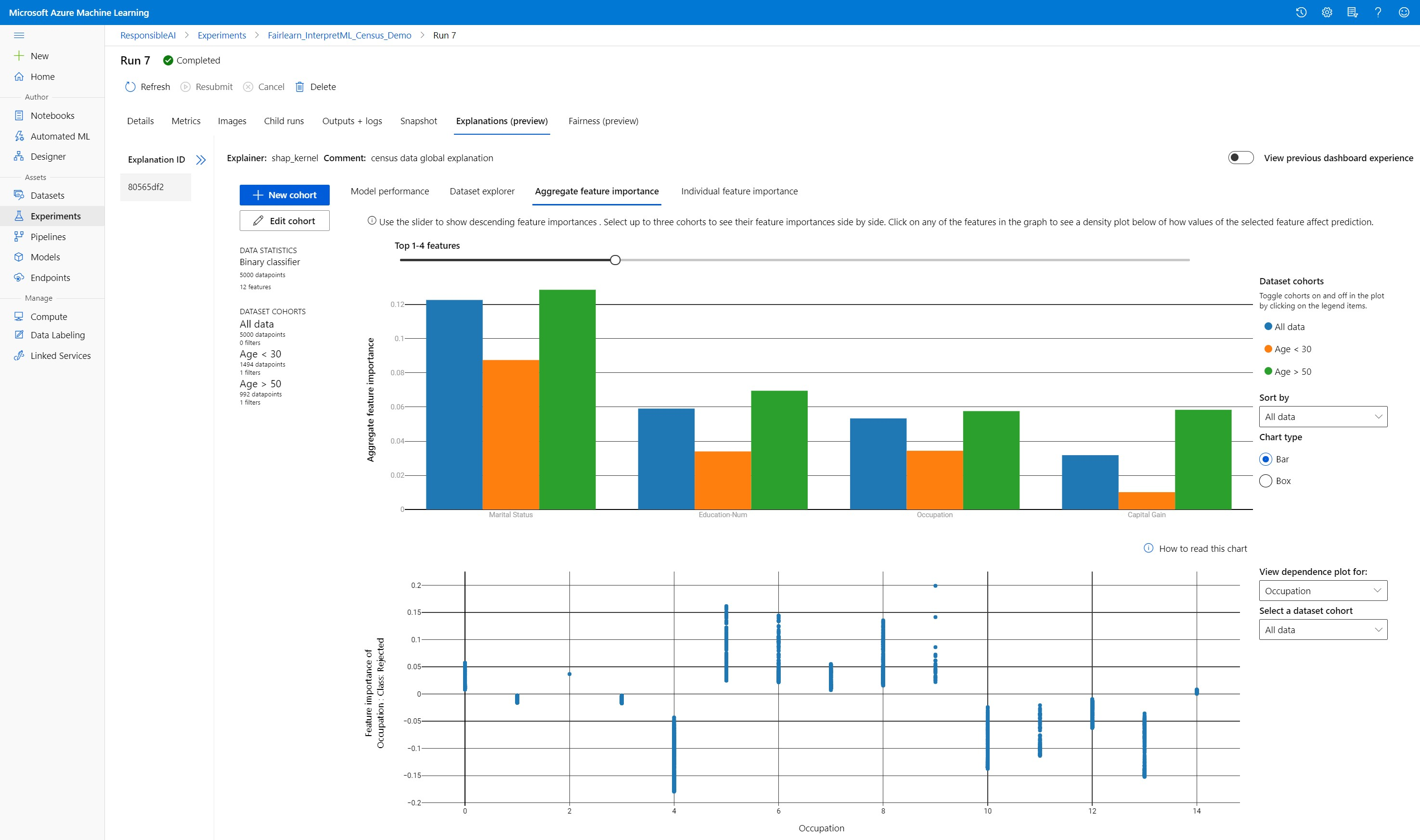
집계 기능 중요도
전반적인 모델 예측에 영향을 주는 상위 K개의 중요한 기능(전역 설명이라고도 함)에 대해 살펴봅니다. 슬라이더를 사용하여 내림차순 기능 중요도 값을 표시합니다. 최대 3개의 코호트를 선택하여 기능 중요도 값을 나란히 표시합니다. 그래프에서 기능 막대를 선택하여 아래 종속성 플롯에서 선택한 기능의 값이 모델 예측에 미치는 영향을 확인합니다.

개별 예측 이해(로컬 설명)
설명 탭의 네 번째 탭에서는 개별 데이터 요소 및 개별 기능 중요도를 자세히 살펴볼 수 있습니다. 주 산점도의 개별 데이터 요소를 클릭하거나 오른쪽의 패널 마법사에서 특정 데이터 요소를 선택하여 모든 데이터 요소에 대한 개별 기능 중요도 플롯을 로드할 수 있습니다.
| 그림 | 설명 |
|---|---|
| 개별 기능 중요도 | 개별 예측에 대한 상위 K개의 중요 기능을 보여 줍니다. 특정 데이터 요소에 대한 기본 모델의 로컬 동작을 설명하는 데 도움이 됩니다. |
| 가상 분석 | 선택한 실제 데이터 요소의 기능 값에 대한 변경 내용을 허용하고 새 기능 값을 사용하는 가상 데이터 요소를 생성하여 예측 값의 변경 결과를 관찰할 수 있습니다. |
| 개별 조건부 기대(ICE) | 최소값에서 최대값으로 기능 값을 변경할 수 있습니다. 기능이 변경될 때 데이터 요소의 예측이 어떻게 변경되는지 설명하는 데 도움이 됩니다. |

참고 항목
이러한 설명은 많은 근사치를 기반으로 하며 예측의 "원인"은 아닙니다. 인과 추론의 엄격한 수학적 견고성 없이 사용자에게 가상 도구의 기능 섭동을 기반으로 실질적인 결정을 내리는 것을 권장하지 않습니다. 이 도구는 주로 모델과 디버깅을 이해하는 데 사용할 수 있습니다.
Azure Machine Learning 스튜디오에서 시각화
원격 해석력 단계(Azure Machine Learning 실행 기록에 생성된 설명 업로드)를 완료하면 Azure Machine Learning 스튜디오의 설명 대시보드에서 시각화를 볼 수 있습니다. 이 대시보드는 Jupyter Notebook 내에서 생성되는 더 간단한 버전의 대시보드 위젯입니다. Azure Machine Learning 스튜디오에는 실시간 계산을 수행할 수 있는 활성 컴퓨팅이 없으므로 가상 데이터 요소 생성 및 ICE 플롯은 사용하지 않도록 설정됩니다.
데이터 세트, 전체 및 로컬 설명을 사용할 수 있는 경우 데이터는 모든 탭을 채웁니다. 그러나 전체 설명만 사용할 수 있는 경우에는 개별 기능 중요도 탭을 사용할 수 없습니다.
다음 경로 중 하나를 따라 Azure Machine Learning 스튜디오의 설명 대시보드에 액세스합니다.
실험 창(미리 보기)
- 왼쪽 창에서 실험을 선택하여 Azure Machine Learning에서 실행한 실험 목록을 확인합니다.
- 특정 실험을 선택하여 해당 실험의 모든 실행을 봅니다.
- 실행을 선택한 다음 설명 탭을 선택하여 설명 시각화 대시보드를 봅니다.
모델 창
- Azure Machine Learning을 사용하여 모델 배포의 단계를 수행하여 원래 모델을 등록한 경우 왼쪽 창에서 모델을 선택하여 볼 수 있습니다.
- 모델을 선택한 다음 설명 탭을 선택하여 설명 대시보드를 봅니다.

유추 시 해석력
원래 모델과 함께 설명을 배포하고 유추 시 이를 사용하여 새 데이터 요소에 대한 개별 기능 중요도 값(로컬 설명)을 제공할 수 있습니다. 또한 유추 시 해석력 성능을 향상시키기 위해 가중치가 낮은 채점 설명자를 제공하며 현재 Azure Machine Learning SDK에서만 지원됩니다. 가중치가 낮은 채점 설명자를 배포하는 프로세스는 모델 배포와 유사하며 다음 단계를 포함합니다.
설명 개체를 만듭니다. 예를 들어
TabularExplainer를 사용할 수 있습니다.from interpret.ext.blackbox import TabularExplainer explainer = TabularExplainer(model, initialization_examples=x_train, features=dataset_feature_names, classes=dataset_classes, transformations=transformations)설명 개체를 사용하여 채점 설명자를 만듭니다.
from azureml.interpret.scoring.scoring_explainer import KernelScoringExplainer, save

# create a lightweight explainer at scoring time
scoring_explainer = KernelScoringExplainer(explainer)

# pickle scoring explainer
# pickle scoring explainer locally
OUTPUT_DIR = 'my_directory'
save(scoring_explainer, directory=OUTPUT_DIR, exist_ok=True)
채점 설명자 모델을 사용하는 이미지를 구성하고 등록합니다.
# register explainer model using the path from ScoringExplainer.save - could be done on remote compute
# scoring_explainer.pkl is the filename on disk, while my_scoring_explainer.pkl will be the filename in cloud storage
run.upload_file('my_scoring_explainer.pkl', os.path.join(OUTPUT_DIR, 'scoring_explainer.pkl'))

scoring_explainer_model = run.register_model(model_name='my_scoring_explainer',
                                             model_path='my_scoring_explainer.pkl')
print(scoring_explainer_model.name, scoring_explainer_model.id, scoring_explainer_model.version, sep = '\t')
선택적 단계로 클라우드에서 채점 설명자를 검색하고 설명을 테스트할 수 있습니다.
from azureml.interpret.scoring.scoring_explainer import load

# retrieve the scoring explainer model from cloud"
scoring_explainer_model = Model(ws, 'my_scoring_explainer')
scoring_explainer_model_path = scoring_explainer_model.download(target_dir=os.getcwd(), exist_ok=True)

# load scoring explainer from disk
scoring_explainer = load(scoring_explainer_model_path)

# test scoring explainer locally
preds = scoring_explainer.explain(x_test)
print(preds)
다음 단계를 수행하여 컴퓨팅 대상에 이미지를 배포합니다.
필요에 따라 Azure Machine Learning을 사용하여 모델 배포의 단계를 수행하여 원래 예측 모델을 등록합니다.
채점 파일을 만듭니다.
%%writefile score.py
import json
import numpy as np
import pandas as pd
import os
import pickle
from sklearn.externals import joblib
from sklearn.linear_model import LogisticRegression
from azureml.core.model import Model

def init():

   global original_model
   global scoring_model

   # retrieve the path to the model file using the model name
   # assume original model is named original_prediction_model
   original_model_path = Model.get_model_path('original_prediction_model')
   scoring_explainer_path = Model.get_model_path('my_scoring_explainer')

   original_model = joblib.load(original_model_path)
   scoring_explainer = joblib.load(scoring_explainer_path)

def run(raw_data):
   # get predictions and explanations for each data point
   data = pd.read_json(raw_data)
   # make prediction
   predictions = original_model.predict(data)
   # retrieve model explanations
   local_importance_values = scoring_explainer.explain(data)
   # you can return any data type as long as it is JSON-serializable
   return {'predictions': predictions.tolist(), 'local_importance_values': local_importance_values}
배포 구성을 정의합니다.
이 구성은 모델 요구 사항에 따라 달라집니다. 다음 예제에서는 하나의 CPU 코어 및 1GB의 메모리를 사용하는 구성을 정의합니다.
from azureml.core.webservice import AciWebservice

 aciconfig = AciWebservice.deploy_configuration(cpu_cores=1,
                                           memory_gb=1,
                                           tags={"data": "NAME_OF_THE_DATASET",
                                                 "method" : "local_explanation"},
                                           description='Get local explanations for NAME_OF_THE_PROBLEM')
환경 종속성을 갖는 파일을 만듭니다.
from azureml.core.conda_dependencies import CondaDependencies

# WARNING: to install this, g++ needs to be available on the Docker image and is not by default (look at the next cell)

azureml_pip_packages = ['azureml-defaults', 'azureml-core', 'azureml-telemetry', 'azureml-interpret']


# specify CondaDependencies obj
myenv = CondaDependencies.create(conda_packages=['scikit-learn', 'pandas'],
                                 pip_packages=['sklearn-pandas'] + azureml_pip_packages,
                                 pin_sdk_version=False)


with open("myenv.yml","w") as f:
   f.write(myenv.serialize_to_string())

with open("myenv.yml","r") as f:
   print(f.read())
g++이 설치된 사용자 지정 Dockerfile을 만듭니다.
%%writefile dockerfile
RUN apt-get update && apt-get install -y g++
만든 이미지를 배포합니다.
이 프로세스는 약 5분이 걸립니다.
from azureml.core.webservice import Webservice
from azureml.core.image import ContainerImage

# use the custom scoring, docker, and conda files we created above
image_config = ContainerImage.image_configuration(execution_script="score.py",
                                                docker_file="dockerfile",
                                                runtime="python",
                                                conda_file="myenv.yml")

# use configs and models generated above
service = Webservice.deploy_from_model(workspace=ws,
                                    name='model-scoring-service',
                                    deployment_config=aciconfig,
                                    models=[scoring_explainer_model, original_model],
                                    image_config=image_config)

service.wait_for_deployment(show_output=True)
배포를 테스트합니다.
import requests

# create data to test service with
examples = x_list[:4]
input_data = examples.to_json()

headers = {'Content-Type':'application/json'}

# send request to service
resp = requests.post(service.scoring_uri, input_data, headers=headers)

print("POST to url", service.scoring_uri)
# can covert back to Python objects from json string if desired
print("prediction:", resp.text)
정리합니다.
배포된 웹 서비스를 삭제하려면
service.delete()를 사용합니다.
문제 해결
스파스 데이터가 지원되지 않음: 모델 설명 대시보드는 많은 기능을 사용하여 중단되거나 속도가 상당히 저하되므로 현재 스파스 데이터 형식을 지원하지 않습니다. 또한 일반적인 메모리 문제는 대량 데이터 세트 및 많은 기능에 발생합니다.
지원되는 설명 기능 매트릭스
| 지원되는 설명 탭 | 원시 기능(밀도 높음) | 원시 기능(스파스) | 엔지니어링된 기능(밀도 높음) | 엔지니어링된 기능(스파스) |
|---|---|---|---|---|
| 모델 성능 | 지원됨(예측 안 함) | 지원됨(예측 안 함) | 지원됨 | 지원됨 |
| 데이터 세트 탐색기 | 지원됨(예측 안 함) | 지원되지 않습니다. 스파스 데이터는 업로드되지 않고 UI에는 스파스 데이터 렌더링 문제가 있습니다. | 지원됨 | 지원되지 않습니다. 스파스 데이터는 업로드되지 않고 UI에는 스파스 데이터 렌더링 문제가 있습니다. |
| 집계 기능 중요도 | 지원됨 | 지원됨 | 지원됨 | 지원됨 |
| 개별 기능 중요도 | 지원됨(예측 안 함) | 지원되지 않습니다. 스파스 데이터는 업로드되지 않고 UI에는 스파스 데이터 렌더링 문제가 있습니다. | 지원됨 | 지원되지 않습니다. 스파스 데이터는 업로드되지 않고 UI에는 스파스 데이터 렌더링 문제가 있습니다. |
모델 설명이 지원되지 않는 예측 모델: 해석력, 최상의 모델 설명은 TCNForecaster, AutoArima, Prophet, ExponentialSmoothing, Average, Naive, Seasonal Average 및 Seasonal Naive 알고리즘을 최고의 모델로 권장하는 AutoML 예측 실험에 사용할 수 없습니다. AutoML 예측 회귀 모델은 설명을 지원합니다. 그러나 설명 대시보드에서는 데이터 파이프라인의 복잡성 때문에 "개별 기능 중요도" 탭이 예측에 대해 지원되지 않습니다.
데이터 인덱스에 대한 로컬 설명: 설명 대시보드는 대시보드가 데이터를 임의로 다운샘플링하므로 데이터 세트가 5000개의 데이터 요소보다 클 경우 원래 유효성 검사 데이터 세트의 행 식별자와 로컬 중요도 값을 연관시키는 것을 지원하지 않습니다. 그러나 대시보드에는 개별 기능 중요도 탭 아래 대시보드에 전달된 각 데이터 요소에 대한 원시 데이터 세트 기능 값이 표시됩니다. 사용자는 원시 데이터 세트 기능 값을 일치시켜 로컬 중요도를 원래 데이터 세트에 다시 매핑할 수 있습니다. 유효성 검사 데이터 세트 크기가 5000개 미만인 경우 Azure Machine Learning 스튜디오의
index기능은 유효성 검사 데이터 세트의 인덱스에 해당합니다.스튜디오에서 가상/ICE 플롯이 지원되지 않음: 업로드된 설명에는 섭동된 기능의 예측과 확률을 다시 계산하기 위해 활성 컴퓨팅이 필요하므로 가상 및 개별 조건부 기대(ICE) 플롯은 Azure Machine Learning 스튜디오에서 지원되지 않습니다. 현재 SDK를 사용하여 위젯으로 실행할 때 Jupyter 노트북에서 지원됩니다.