레시피: Azure AI 서비스 - 다변량 변칙 검색
이 레시피는 다변량 변칙 검색을 위해 Apache Spark에서 SynapseML 및 Azure AI 서비스를 사용하는 방법을 보여 줍니다. 다변량 변칙 검색을 사용하면 다양한 변수 간의 모든 상관 관계 및 종속성을 고려하여 많은 변수 또는 시계열 간의 변칙을 검색할 수 있습니다. 이 시나리오에서는 SynapseML을 사용하여 Azure AI 서비스를 사용하여 다변량 변칙 검색을 위한 모델을 학습한 다음, 모델을 사용하여 3개의 IoT 센서에서 가상 측정을 포함하는 데이터 세트 내에서 다변량 변칙을 유추합니다.
Important
2023년 9월 20일부터 새 Anomaly Detector 리소스를 만들 수 없습니다. Anomaly Detector 서비스는 2026년 10월 1일에 사용 중지됩니다.
Azure AI Anomaly Detector에 대한 자세한 내용은 이 설명서 페이지를 참조 하세요.
필수 조건
- Azure 구독 - 체험 구독 만들기
- 레이크하우스에 전자 필기장을 첨부합니다. 왼쪽에서 추가를 선택하여 기존 레이크하우스를 추가하거나 레이크하우스를 만듭니다.
설정
지침에 따라 Azure Portal을 사용하여 리소스를 Anomaly Detector 만들거나 Azure CLI를 사용하여 이 리소스를 만들 수도 있습니다.
설정한 Anomaly Detector후 다양한 양식의 데이터를 처리하는 방법을 탐색할 수 있습니다. Azure AI 내의 서비스 카탈로그는 비전, 음성, 언어, 웹 검색, 의사 결정, 번역 및 문서 인텔리전스와 같은 몇 가지 옵션을 제공합니다.
Anomaly Detector 리소스 만들기
- Azure Portal에서 리소스 그룹에서 만들기를 선택한 다음 Anomaly Detector를 입력 합니다. Anomaly Detector 리소스를 선택합니다.
- 리소스에 이름을 지정하고 리소스 그룹의 나머지 부분과 동일한 지역을 사용하는 것이 좋습니다. 나머지에 대한 기본 옵션을 사용한 다음 검토 + 만들기를 선택한 다음 만들기를 선택합니다.
- Anomaly Detector 리소스가 만들어지면 해당 리소스를 열고 왼쪽 탐색에서 패널을 선택합니다
Keys and Endpoints. Anomaly Detector 리소스의 키를 환경 변수에ANOMALY_API_KEY복사하거나 변수에anomalyKey저장합니다.
Storage 계정 리소스 만들기
중간 데이터를 저장하려면 Azure Blob Storage 계정을 만들어야 합니다. 해당 스토리지 계정 내에서 중간 데이터를 저장하기 위한 컨테이너를 만듭니다. 컨테이너 이름을 기록하고 해당 컨테이너에 연결 문자열 복사합니다. 나중에 변수와 BLOB_CONNECTION_STRING 환경 변수를 containerName 채우는 데 필요합니다.
서비스 키 입력
먼저 서비스 키에 대한 환경 변수를 설정해 보겠습니다. 다음 셀은 Azure Key Vault에 BLOB_CONNECTION_STRING 저장된 값을 기반으로 환경 변수 및 환경 변수를 설정합니다ANOMALY_API_KEY. 사용자 고유의 환경에서 이 자습서를 실행하는 경우 계속하기 전에 이러한 환경 변수를 설정해야 합니다.
import os
from pyspark.sql import SparkSession
from synapse.ml.core.platform import find_secret

# Bootstrap Spark Session
spark = SparkSession.builder.getOrCreate()
이제 환경 변수 및 BLOB_CONNECTION_STRING 환경 변수를 ANOMALY_API_KEY 읽고 변수 및 location 변수를 containerName 설정할 수 있습니다.
# An Anomaly Dectector subscription key
anomalyKey = find_secret("anomaly-api-key") # use your own anomaly api key
# Your storage account name
storageName = "anomalydetectiontest" # use your own storage account name
# A connection string to your blob storage account
storageKey = find_secret("madtest-storage-key") # use your own storage key
# A place to save intermediate MVAD results
intermediateSaveDir = (
    "wasbs://madtest@anomalydetectiontest.blob.core.windows.net/intermediateData"
)
# The location of the anomaly detector resource that you created
location = "westus2"
먼저 변칙 탐지기가 중간 결과를 저장할 수 있도록 스토리지 계정에 연결합니다.
spark.sparkContext._jsc.hadoopConfiguration().set(
    f"fs.azure.account.key.{storageName}.blob.core.windows.net", storageKey
)
필요한 모든 모듈을 가져오겠습니다.
import numpy as np
import pandas as pd

import pyspark
from pyspark.sql.functions import col
from pyspark.sql.functions import lit
from pyspark.sql.types import DoubleType
import matplotlib.pyplot as plt

import synapse.ml
from synapse.ml.cognitive import *
이제 샘플 데이터를 Spark DataFrame으로 읽어 보겠습니다.
df = (
    spark.read.format("csv")
    .option("header", "true")
    .load("wasbs://publicwasb@mmlspark.blob.core.windows.net/MVAD/sample.csv")
)

df = (
    df.withColumn("sensor_1", col("sensor_1").cast(DoubleType()))
    .withColumn("sensor_2", col("sensor_2").cast(DoubleType()))
    .withColumn("sensor_3", col("sensor_3").cast(DoubleType()))
)

# Let's inspect the dataframe:
df.show(5)
이제 모델을 학습시키는 estimator 데 사용되는 개체를 만들 수 있습니다. 학습 데이터의 시작 및 종료 시간을 지정합니다. 사용할 입력 열과 타임스탬프가 포함된 열의 이름도 지정합니다. 마지막으로 변칙 검색 슬라이딩 윈도우에서 사용할 데이터 포인트 수를 지정하고 연결 문자열 Azure Blob Storage 계정으로 설정합니다.
trainingStartTime = "2020-06-01T12:00:00Z"
trainingEndTime = "2020-07-02T17:55:00Z"
timestampColumn = "timestamp"
inputColumns = ["sensor_1", "sensor_2", "sensor_3"]

estimator = (
    FitMultivariateAnomaly()
    .setSubscriptionKey(anomalyKey)
    .setLocation(location)
    .setStartTime(trainingStartTime)
    .setEndTime(trainingEndTime)
    .setIntermediateSaveDir(intermediateSaveDir)
    .setTimestampCol(timestampColumn)
    .setInputCols(inputColumns)
    .setSlidingWindow(200)
)
이제 데이터를 만들었 estimator으므로 데이터에 맞추겠습니다.
model = estimator.fit(df)
```parameter

Once the training is done, we can now use the model for inference. The code in the next cell specifies the start and end times for the data we would like to detect the anomalies in.

```python
inferenceStartTime = "2020-07-02T18:00:00Z"
inferenceEndTime = "2020-07-06T05:15:00Z"

result = (
    model.setStartTime(inferenceStartTime)
    .setEndTime(inferenceEndTime)
    .setOutputCol("results")
    .setErrorCol("errors")
    .setInputCols(inputColumns)
    .setTimestampCol(timestampColumn)
    .transform(df)
)

result.show(5)
이전 셀에서 호출 .show(5) 했을 때 데이터 프레임의 처음 5개 행이 표시됩니다. 결과는 null 모두 유추 창 내에 없었기 때문입니다.
유추된 데이터에 대해서만 결과를 표시하려면 필요한 열을 선택할 수 있습니다. 그런 다음 오름차순으로 데이터 프레임의 행을 정렬하고 결과를 필터링하여 유추 창 범위에 있는 행만 표시할 수 있습니다. 이 경우 inferenceEndTime 데이터 프레임의 마지막 행과 동일하므로 무시할 수 있습니다.
마지막으로 결과를 더 잘 그릴 수 있도록 Spark 데이터 프레임을 Pandas 데이터 프레임으로 변환할 수 있습니다.
rdf = (
    result.select(
        "timestamp",
        *inputColumns,
        "results.contributors",
        "results.isAnomaly",
        "results.severity"
    )
    .orderBy("timestamp", ascending=True)
    .filter(col("timestamp") >= lit(inferenceStartTime))
    .toPandas()
)

rdf
각 센서의 contributors 기여 점수를 저장하는 열의 형식을 검색된 변칙으로 지정합니다. 다음 셀은 이 데이터의 서식을 지정하고 각 센서의 기여 점수를 자체 열로 분할합니다.
def parse(x):
    if type(x) is list:
        return dict([item[::-1] for item in x])
    else:
        return {"series_0": 0, "series_1": 0, "series_2": 0}

rdf["contributors"] = rdf["contributors"].apply(parse)
rdf = pd.concat(
    [rdf.drop(["contributors"], axis=1), pd.json_normalize(rdf["contributors"])], axis=1
)
rdf
좋습니다! 이제 각각 센서 1, 2, 3 및 series_2 열의 series_0series_1기여 점수가 있습니다.
다음 셀을 실행하여 결과를 표시합니다. 매개 변수는 minSeverity 표시할 변칙의 최소 심각도를 지정합니다.
minSeverity = 0.1

####### Main Figure #######
plt.figure(figsize=(23, 8))
plt.plot(
    rdf["timestamp"],
    rdf["sensor_1"],
    color="tab:orange",
    linestyle="solid",
    linewidth=2,
    label="sensor_1",
)
plt.plot(
    rdf["timestamp"],
    rdf["sensor_2"],
    color="tab:green",
    linestyle="solid",
    linewidth=2,
    label="sensor_2",
)
plt.plot(
    rdf["timestamp"],
    rdf["sensor_3"],
    color="tab:blue",
    linestyle="solid",
    linewidth=2,
    label="sensor_3",
)
plt.grid(axis="y")
plt.tick_params(axis="x", which="both", bottom=False, labelbottom=False)
plt.legend()

anoms = list(rdf["severity"] >= minSeverity)
_, _, ymin, ymax = plt.axis()
plt.vlines(np.where(anoms), ymin=ymin, ymax=ymax, color="r", alpha=0.8)

plt.legend()
plt.title(
    "A plot of the values from the three sensors with the detected anomalies highlighted in red."
)
plt.show()

####### Severity Figure #######
plt.figure(figsize=(23, 1))
plt.tick_params(axis="x", which="both", bottom=False, labelbottom=False)
plt.plot(
    rdf["timestamp"],
    rdf["severity"],
    color="black",
    linestyle="solid",
    linewidth=2,
    label="Severity score",
)
plt.plot(
    rdf["timestamp"],
    [minSeverity] * len(rdf["severity"]),
    color="red",
    linestyle="dotted",
    linewidth=1,
    label="minSeverity",
)
plt.grid(axis="y")
plt.legend()
plt.ylim([0, 1])
plt.title("Severity of the detected anomalies")
plt.show()

####### Contributors Figure #######
plt.figure(figsize=(23, 1))
plt.tick_params(axis="x", which="both", bottom=False, labelbottom=False)
plt.bar(
    rdf["timestamp"], rdf["series_0"], width=2, color="tab:orange", label="sensor_1"
)
plt.bar(
    rdf["timestamp"],
    rdf["series_1"],
    width=2,
    color="tab:green",
    label="sensor_2",
    bottom=rdf["series_0"],
)
plt.bar(
    rdf["timestamp"],
    rdf["series_2"],
    width=2,
    color="tab:blue",
    label="sensor_3",
    bottom=rdf["series_0"] + rdf["series_1"],
)
plt.grid(axis="y")
plt.legend()
plt.ylim([0, 1])
plt.title("The contribution of each sensor to the detected anomaly")
plt.show()
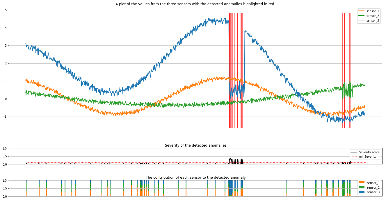
그림에는 센서의 원시 데이터(유추 창 내부)가 주황색, 녹색 및 파란색으로 표시됩니다. 첫 번째 그림의 빨간색 세로선은 심각도가 1보다 크거나 같은 검색된 변칙을 minSeverity보여줍니다.
두 번째 플롯은 검색된 모든 변칙의 심각도 점수를 보여 하며 임계값은 minSeverity 점선 빨간색 선에 표시됩니다.
마지막으로, 마지막 플롯은 각 센서에서 검색된 변칙에 대한 데이터의 기여도를 보여 줍니다. 각 변칙의 가장 가능성이 큰 원인을 진단하고 이해하는 데 도움이 됩니다.
관련 콘텐츠
피드백
출시 예정: 2024년 내내 콘텐츠에 대한 피드백 메커니즘으로 GitHub 문제를 단계적으로 폐지하고 이를 새로운 피드백 시스템으로 바꿀 예정입니다. 자세한 내용은 다음을 참조하세요. https://aka.ms/ContentUserFeedback
다음에 대한 사용자 의견 제출 및 보기