적용 대상:![]() SQL Server 2017(14.x) 이상 버전
SQL Server 2017(14.x) 이상 버전
이 문서에서는 SQL Server Machine Learning Services에서 외부 Python 스크립트를 실행하기 위한 Python 확장에 대해 설명합니다. 이 확장은 다음을 추가합니다.
- Python 실행 환경
- Python 3.5 런타임 및 인터프리터를 사용한 Anaconda 배포판
- 표준 라이브러리 및 도구
- Microsoft Python 패키지:
- 대규모 분석을 위한 revoscalepy
- 기계 학습 알고리즘을 위한 microsoftml
Python 3.5 런타임 및 인터프리터를 설치하면 표준 Python 솔루션과 거의 완벽한 호환성이 보장됩니다. Python은 SQL Server와 별도의 프로세스에서 실행되어 데이터베이스 작업이 손상되지 않도록 보장합니다.
Python 구성 요소
SQL Server는 오픈 소스 패키지와 독점 패키지를 모두 포함하고 있습니다. 설치 프로그램에서 설치하는 Python 런타임은 Python 3.5가 포함된 Anaconda 4.2입니다. Python 런타임은 SQL 도구와 독립적으로 설치되며, 핵심 엔진 프로세스 외부인 확장성 프레임워크에서 실행됩니다. Python을 사용하여 Machine Learning Services를 설치하는 과정의 일환으로 GNU 공개 라이선스 조건에 동의해야 합니다.
SQL Server는 Python 실행 파일을 수정하지 않지만 해당 버전은 독점 패키지가 빌드되고 테스트되는 버전이므로 설치 프로그램에서 설치한 Python 버전을 사용해야 합니다. Anaconda 배포판에서 지원하는 패키지 목록은 Continuum 분석 사이트: Anaconda 패키지 목록을 참조하세요.
특정 데이터베이스 엔진 인스턴스와 연결된 Anaconda 배포판은 인스턴스와 연결된 폴더에서 찾을 수 있습니다. 예를 들어 기본 인스턴스에 Machine Learning Services 및 Python을 사용하여 SQL Server 2017 데이터베이스 엔진을 설치한 경우 C:\Program Files\Microsoft SQL Server\MSSQL14.MSSQLSERVER\PYTHON_SERVICES 아래를 확인하세요.
병렬 및 분산 워크로드를 처리하기 위해 Microsoft에서 추가한 Python 패키지에는 다음 라이브러리가 포함되어 있습니다.
| 라이브러리 | 설명 |
|---|---|
| revoscalepy | 데이터 원본 개체와 데이터 탐색, 조작, 변환 및 시각화를 지원합니다. rxLinMod와 같이 다양한 확장 가능한 기계 학습 모델뿐 아니라 원격 컴퓨팅 컨텍스트 만들기도 지원합니다. 자세한 내용은 SQL Server와 revoscalepy 모듈을 참조하세요. |
| microsoftml | 속도와 정확도에 최적화된 기계 학습 알고리즘과 텍스트 및 이미지 작업을 위한 인라인 변환이 포함되어 있습니다. 자세한 내용은 SQL Server의 microsoftml 모듈을 참조하세요. |
Microsoftml과 revoscalepy는 긴밀하게 결합되어 있으며, microsoftml에서 사용되는 데이터 원본은 revoscalepy 개체로 정의됩니다. revoscalepy에서 컴퓨팅 컨텍스트 제한을 microsoftml로 전환합니다. 즉, 모든 기능을 로컬 작업에 사용할 수 있지만 원격 컴퓨팅 컨텍스트로 전환하려면 RxInSqlServer가 필요합니다.
SQL Server에서 Python 사용
revoscalepy 모듈을 Python 코드로 가져온 다음, 다른 Python 함수와 마찬가지로 모듈에서 함수를 호출합니다.
지원되는 데이터 원본으로는 ODBC 데이터베이스, SQL Server, 그리고 다른 원본 또는 R 솔루션과 데이터를 교환할 수 있는 XDF 파일 형식이 있습니다. Python의 입력 데이터는 테이블 형식이어야 합니다. 모든 Python 결과는 pandas 데이터 프레임 형식으로 반환되어야 합니다.
지원되는 컴퓨팅 컨텍스트로는 로컬 또는 원격 SQL Server 컴퓨팅 컨텍스트가 있습니다. 원격 컴퓨팅 컨텍스트는 워크스테이션 같은 한 컴퓨터에서 시작하는 코드 실행을 참조하지만, 이후에 스크립트 실행을 원격 컴퓨터로 전환합니다. 컴퓨팅 컨텍스트를 전환하려면 두 시스템의 revoscalepy 라이브러리가 동일해야 합니다.
예상하시겠지만, 로컬 컴퓨팅 컨텍스트에는 데이터베이스 엔진 인스턴스와 동일한 서버에서 실행되는 Python 코드와 T-SQL 내 또는 저장 프로시저에 포함된 코드가 들어 있습니다. 또한 원격 컴퓨팅 컨텍스트를 정의하여 로컬 Python IDE에서 코드를 실행하고 SQL Server 컴퓨터에서 스크립트를 실행할 수 있습니다.
실행 아키텍처
다음 다이어그램은 SQL Server 컴퓨팅 컨텍스트를 사용하여 지원되는 각 시나리오(데이터베이스 내에서 스크립트 실행, Python 터미널에서 원격 실행)에서 SQL Server 구성 요소와 Python 런타임 간에 이루어지는 상호 작용을 보여줍니다.
데이터베이스 내에서 실행되는 Python 스크립트
SQL Server ‘내부’에서 Python을 실행하는 경우 특수 저장 프로시저 sp_execute_external_script 내부에 Python 스크립트를 캡슐화해야 합니다.
저장 프로시저에 스크립트가 포함된 후에는 저장 프로시저 호출을 수행할 수 있는 애플리케이션에서 Python 코드 실행을 시작할 수 있습니다. 이후 SQL Server는 다음 다이어그램에 요약된 대로 코드 실행을 관리합니다.
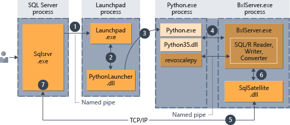
- Python 런타임에 대한 요청은 저장 프로시저에 전달된 매개 변수
@language='Python'으로 표시됩니다. SQL Server는 실행 패드 서비스에 이 요청을 보냅니다. Linux에서 SQL은 실행 패드 서비스를 사용하여 각 사용자에 대한 별도의 실행 패드 프로세스와 통신합니다. 자세한 내용은 확장성 아키텍처 다이어그램을 참조하세요. - 실행 패드 서비스가 적절한 시작 관리자(여기서는 PythonLauncher)를 시작합니다.
- PythonLauncher는 외부 Python35 프로세스를 시작합니다.
- BxlServer는 Python 런타임과 조율하여 데이터 교환 및 작업 결과 저장을 관리합니다.
- SQL Satellite는 SQL Server를 사용하여 관련 작업 및 프로세스에 대한 통신을 관리합니다.
- BxlServer는 SQL Satellite를 사용하여 상태 및 결과를 SQL Server에 전달합니다.
- SQL Server는 결과를 얻고 관련 작업과 프로세스를 닫습니다.
원격 클라이언트에서 실행되는 Python 스크립트
다음 조건이 충족되는 경우 노트북과 같은 원격 컴퓨터에서 Python 스크립트를 실행하고 SQL Server 컴퓨터의 컨텍스트에서 실행할 수 있습니다.
- 스크립트를 적절하게 설계합니다.
- 원격 컴퓨터에 Machine Learning Services에서 사용되는 확장성 라이브러리가 설치되어 있습니다. revoscalepy 패키지는 원격 컴퓨팅 컨텍스트를 사용하는 데 필요합니다.
다음 다이어그램은 원격 컴퓨터에서 스크립트가 전송될 때의 전체 워크플로를 요약한 것입니다.
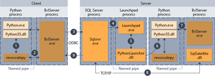
- revoscalepy에서 지원되는 함수의 경우 Python 런타임은 BxlServer를 호출하는 연결 함수를 호출합니다.
- BxlServer는 Machine Learning Services(데이터베이스 내)에 포함되어 있으며 Python 런타임과는 별도의 프로세스에서 실행됩니다.
- BxlServer가 연결 대상을 결정하고 ODBC를 통해 연결을 시작한 다음, Python 스크립트에 연결 문자열의 일부로 제공된 자격 증명을 전달합니다.
- BxlServer가 SQL Server 인스턴스에 대한 연결을 엽니다.
- 외부 스크립트 런타임이 호출되면 실행 패드 서비스가 호출되고, 실행 패드 서비스는 적절한 시작 관리자(여기서는 PythonLauncher)를 시작합니다. 그 후 Python 코드 처리는 T-SQL의 저장 프로시저에서 Python 코드를 호출할 때와 유사한 워크플로에서 처리됩니다.
- PythonLauncher는 SQL Server 컴퓨터에 설치된 Python 런타임의 인스턴스를 호출합니다.
- 결과가 BxlServer로 반환됩니다.
- SQL Satellite가 SQL Server와의 통신과 관련 작업 개체 정리를 관리합니다.
- SQL Server가 클라이언트에 결과를 전달합니다.