연습 - 실제 문제에 대한 리소스 예측 - Training

10분

Shor의 팩터링 알고리즘은 가장 잘 알려진 양자 알고리즘 중 하나입니다. 알려진 클래식 팩터링 알고리즘에 대한 기하급수적 속도 향상을 제공합니다.

클래식 암호화는 계산 난이도와 같은 물리적 또는 수학적 수단을 사용하여 작업을 수행합니다. 인기 있는 암호화 프로토콜은 리베스트-샤미르-Adleman(RSA) 체계로, 클래식 컴퓨터를 사용하여 소수를 계산하는 데 어려움이 있다는 가정하에 사용됩니다.

Shor 알고리즘은 충분히 큰 양자 컴퓨터가 공개 키 암호화를 끊을 수 있음을 의미합니다. Shor의 알고리즘에 필요한 리소스를 예측하는 것은 이러한 유형의 암호화 체계의 취약성을 평가하는 데 중요합니다.

다음 연습에서는 2048비트 정수의 인수분해에 대한 리소스 예측을 계산합니다. 이 애플리케이션의 경우 사전 계산된 논리 리소스 예측으로부터 직접 실제 리소스 추정치를 계산합니다. 허용되는 오류 예산의 경우 $\epsilon = 1/3$를 사용합니다.

Shor 알고리즘 작성

VS Code에서 명령 팔레트 보기를 > 선택하고 만들기: 새 Jupyter Notebook을 선택합니다.
Notebook을 ShorRE.ipynb으로 저장합니다.
Notebook의 첫 번째 셀에서 패키지를 가져옵니다 qsharp .
```
import qsharp
```

네임스페이 Microsoft.Quantum.ResourceEstimation 스를 사용하여 Shor의 정수 팩터리화 알고리즘의 캐시되고 최적화된 버전을 정의합니다. 새 셀을 추가하고 다음 코드를 복사합니다.

%%qsharp
open Microsoft.Quantum.Arrays;
open Microsoft.Quantum.Canon;
open Microsoft.Quantum.Convert;
open Microsoft.Quantum.Diagnostics;
open Microsoft.Quantum.Intrinsic;
open Microsoft.Quantum.Math;
open Microsoft.Quantum.Measurement;
open Microsoft.Quantum.Unstable.Arithmetic;
open Microsoft.Quantum.ResourceEstimation;

operation RunProgram() : Unit {
    let bitsize = 31;

    // When choosing parameters for `EstimateFrequency`, make sure that
    // generator and modules are not co-prime
    let _ = EstimateFrequency(11, 2^bitsize - 1, bitsize);
}


// In this sample we concentrate on costing the `EstimateFrequency`
// operation, which is the core quantum operation in Shors algorithm, and
// we omit the classical pre- and post-processing.

/// # Summary
/// Estimates the frequency of a generator
/// in the residue ring Z mod `modulus`.
///
/// # Input
/// ## generator
/// The unsigned integer multiplicative order (period)
/// of which is being estimated. Must be co-prime to `modulus`.
/// ## modulus
/// The modulus which defines the residue ring Z mod `modulus`
/// in which the multiplicative order of `generator` is being estimated.
/// ## bitsize
/// Number of bits needed to represent the modulus.
///
/// # Output
/// The numerator k of dyadic fraction k/2^bitsPrecision
/// approximating s/r.
operation EstimateFrequency(
    generator : Int,
    modulus : Int,
    bitsize : Int
)
: Int {
    mutable frequencyEstimate = 0;
    let bitsPrecision =  2 * bitsize + 1;

    // Allocate qubits for the superposition of eigenstates of
    // the oracle that is used in period finding.
    use eigenstateRegister = Qubit[bitsize];

    // Initialize eigenstateRegister to 1, which is a superposition of
    // the eigenstates we are estimating the phases of.
    // We first interpret the register as encoding an unsigned integer
    // in little endian encoding.
    ApplyXorInPlace(1, eigenstateRegister);
    let oracle = ApplyOrderFindingOracle(generator, modulus, _, _);

    // Use phase estimation with a semiclassical Fourier transform to
    // estimate the frequency.
    use c = Qubit();
    for idx in bitsPrecision - 1..-1..0 {
        within {
            H(c);
        } apply {
            // `BeginEstimateCaching` and `EndEstimateCaching` are the operations
            // exposed by Azure Quantum Resource Estimator. These will instruct
            // resource counting such that the if-block will be executed
            // only once, its resources will be cached, and appended in
            // every other iteration.
            if BeginEstimateCaching("ControlledOracle", SingleVariant()) {
                Controlled oracle([c], (1 <<< idx, eigenstateRegister));
                EndEstimateCaching();
            }
            R1Frac(frequencyEstimate, bitsPrecision - 1 - idx, c);
        }
        if MResetZ(c) == One {
            set frequencyEstimate += 1 <<< (bitsPrecision - 1 - idx);
        }
    }

    // Return all the qubits used for oracles eigenstate back to 0 state
    // using Microsoft.Quantum.Intrinsic.ResetAll.
    ResetAll(eigenstateRegister);

    return frequencyEstimate;
}

/// # Summary
/// Interprets `target` as encoding unsigned little-endian integer k
/// and performs transformation |k⟩ ↦ |gᵖ⋅k mod N ⟩ where
/// p is `power`, g is `generator` and N is `modulus`.
///
/// # Input
/// ## generator
/// The unsigned integer multiplicative order ( period )
/// of which is being estimated. Must be co-prime to `modulus`.
/// ## modulus
/// The modulus which defines the residue ring Z mod `modulus`
/// in which the multiplicative order of `generator` is being estimated.
/// ## power
/// Power of `generator` by which `target` is multiplied.
/// ## target
/// Register interpreted as LittleEndian which is multiplied by
/// given power of the generator. The multiplication is performed modulo
/// `modulus`.
internal operation ApplyOrderFindingOracle(
    generator : Int, modulus : Int, power : Int, target : Qubit[]
)
: Unit
is Adj + Ctl {
    // The oracle we use for order finding implements |x⟩ ↦ |x⋅a mod N⟩. We
    // also use `ExpModI` to compute a by which x must be multiplied. Also
    // note that we interpret target as unsigned integer in little-endian
    // encoding by using the `LittleEndian` type.
    ModularMultiplyByConstant(modulus,
                                ExpModI(generator, power, modulus),
                                target);
}

/// # Summary
/// Performs modular in-place multiplication by a classical constant.
///
/// # Description
/// Given the classical constants `c` and `modulus`, and an input
/// quantum register (as LittleEndian) |𝑦⟩, this operation
/// computes `(c*x) % modulus` into |𝑦⟩.
///
/// # Input
/// ## modulus
/// Modulus to use for modular multiplication
/// ## c
/// Constant by which to multiply |𝑦⟩
/// ## y
/// Quantum register of target
internal operation ModularMultiplyByConstant(modulus : Int, c : Int, y : Qubit[])
: Unit is Adj + Ctl {
    use qs = Qubit[Length(y)];
    for (idx, yq) in Enumerated(y) {
        let shiftedC = (c <<< idx) % modulus;
        Controlled ModularAddConstant([yq], (modulus, shiftedC, qs));
    }
    ApplyToEachCA(SWAP, Zipped(y, qs));
    let invC = InverseModI(c, modulus);
    for (idx, yq) in Enumerated(y) {
        let shiftedC = (invC <<< idx) % modulus;
        Controlled ModularAddConstant([yq], (modulus, modulus - shiftedC, qs));
    }
}

/// # Summary
/// Performs modular in-place addition of a classical constant into a
/// quantum register.
///
/// # Description
/// Given the classical constants `c` and `modulus`, and an input
/// quantum register (as LittleEndian) |𝑦⟩, this operation
/// computes `(x+c) % modulus` into |𝑦⟩.
///
/// # Input
/// ## modulus
/// Modulus to use for modular addition
/// ## c
/// Constant to add to |𝑦⟩
/// ## y
/// Quantum register of target
internal operation ModularAddConstant(modulus : Int, c : Int, y : Qubit[])
: Unit is Adj + Ctl {
    body (...) {
        Controlled ModularAddConstant([], (modulus, c, y));
    }
    controlled (ctrls, ...) {
        // We apply a custom strategy to control this operation instead of
        // letting the compiler create the controlled variant for us in which
        // the `Controlled` functor would be distributed over each operation
        // in the body.
        //
        // Here we can use some scratch memory to save ensure that at most one
        // control qubit is used for costly operations such as `AddConstant`
        // and `CompareGreaterThenOrEqualConstant`.
        if Length(ctrls) >= 2 {
            use control = Qubit();
            within {
                Controlled X(ctrls, control);
            } apply {
                Controlled ModularAddConstant([control], (modulus, c, y));
            }
        } else {
            use carry = Qubit();
            Controlled AddConstant(ctrls, (c, y + [carry]));
            Controlled Adjoint AddConstant(ctrls, (modulus, y + [carry]));
            Controlled AddConstant([carry], (modulus, y));
            Controlled CompareGreaterThanOrEqualConstant(ctrls, (c, y, carry));
        }
    }
}

/// # Summary
/// Performs in-place addition of a constant into a quantum register.
///
/// # Description
/// Given a non-empty quantum register |𝑦⟩ of length 𝑛+1 and a positive
/// constant 𝑐 < 2ⁿ, computes |𝑦 + c⟩ into |𝑦⟩.
///
/// # Input
/// ## c
/// Constant number to add to |𝑦⟩.
/// ## y
/// Quantum register of second summand and target; must not be empty.
internal operation AddConstant(c : Int, y : Qubit[]) : Unit is Adj + Ctl {
    // We are using this version instead of the library version that is based
    // on Fourier angles to show an advantage of sparse simulation in this sample.

    let n = Length(y);
    Fact(n > 0, "Bit width must be at least 1");

    Fact(c >= 0, "constant must not be negative");
    Fact(c < 2 ^ n, $"constant must be smaller than {2L ^ n}");

    if c != 0 {
        // If c has j trailing zeroes than the j least significant bits
        // of y will not be affected by the addition and can therefore be
        // ignored by applying the addition only to the other qubits and
        // shifting c accordingly.
        let j = NTrailingZeroes(c);
        use x = Qubit[n - j];
        within {
            ApplyXorInPlace(c >>> j, x);
        } apply {
            IncByLE(x, y[j...]);
        }
    }
}

/// # Summary
/// Performs greater-than-or-equals comparison to a constant.
///
/// # Description
/// Toggles output qubit `target` if and only if input register `x`
/// is greater than or equal to `c`.
///
/// # Input
/// ## c
/// Constant value for comparison.
/// ## x
/// Quantum register to compare against.
/// ## target
/// Target qubit for comparison result.
///
/// # Reference
/// This construction is described in [Lemma 3, arXiv:2201.10200]
internal operation CompareGreaterThanOrEqualConstant(c : Int, x : Qubit[], target : Qubit)
: Unit is Adj+Ctl {
    let bitWidth = Length(x);

    if c == 0 {
        X(target);
    } elif c >= 2 ^ bitWidth {
        // do nothing
    } elif c == 2 ^ (bitWidth - 1) {
        ApplyLowTCNOT(Tail(x), target);
    } else {
        // normalize constant
        let l = NTrailingZeroes(c);

        let cNormalized = c >>> l;
        let xNormalized = x[l...];
        let bitWidthNormalized = Length(xNormalized);
        let gates = Rest(IntAsBoolArray(cNormalized, bitWidthNormalized));

        use qs = Qubit[bitWidthNormalized - 1];
        let cs1 = [Head(xNormalized)] + Most(qs);
        let cs2 = Rest(xNormalized);

        within {
            for i in IndexRange(gates) {
                (gates[i] ? ApplyAnd | ApplyOr)(cs1[i], cs2[i], qs[i]);
            }
        } apply {
            ApplyLowTCNOT(Tail(qs), target);
        }
    }
}

/// # Summary
/// Internal operation used in the implementation of GreaterThanOrEqualConstant.
internal operation ApplyOr(control1 : Qubit, control2 : Qubit, target : Qubit) : Unit is Adj {
    within {
        ApplyToEachA(X, [control1, control2]);
    } apply {
        ApplyAnd(control1, control2, target);
        X(target);
    }
}

internal operation ApplyAnd(control1 : Qubit, control2 : Qubit, target : Qubit)
: Unit is Adj {
    body (...) {
        CCNOT(control1, control2, target);
    }
    adjoint (...) {
        H(target);
        if (M(target) == One) {
            X(target);
            CZ(control1, control2);
        }
    }
}


/// # Summary
/// Returns the number of trailing zeroes of a number
///
/// ## Example
/// ```qsharp
/// let zeroes = NTrailingZeroes(21); // = NTrailingZeroes(0b1101) = 0
/// let zeroes = NTrailingZeroes(20); // = NTrailingZeroes(0b1100) = 2
/// ```
internal function NTrailingZeroes(number : Int) : Int {
    mutable nZeroes = 0;
    mutable copy = number;
    while (copy % 2 == 0) {
        set nZeroes += 1;
        set copy /= 2;
    }
    return nZeroes;
}

/// # Summary
/// An implementation for `CNOT` that when controlled using a single control uses
/// a helper qubit and uses `ApplyAnd` to reduce the T-count to 4 instead of 7.
internal operation ApplyLowTCNOT(a : Qubit, b : Qubit) : Unit is Adj+Ctl {
    body (...) {
        CNOT(a, b);
    }

    adjoint self;

    controlled (ctls, ...) {
        // In this application this operation is used in a way that
        // it is controlled by at most one qubit.
        Fact(Length(ctls) <= 1, "At most one control line allowed");

        if IsEmpty(ctls) {
            CNOT(a, b);
        } else {
            use q = Qubit();
            within {
                ApplyAnd(Head(ctls), a, q);
            } apply {
                CNOT(q, b);
            }
        }
    }

    controlled adjoint self;
}

Shor 알고리즘 예측

이제 기본 가정을 사용하여 작업에 대한 RunProgram 실제 리소스를 예측합니다. 새 셀을 추가하고 다음 코드를 복사합니다.

result = qsharp.estimate("RunProgram()")
result

이 함수는 qsharp.estimate 전체 물리적 리소스 수가 있는 테이블을 표시하는 데 사용할 수 있는 결과 개체를 만듭니다. 더 많은 정보가 있는 그룹을 축소해 비용 세부 정보를 검사할 수 있습니다.

예를 들어 논리 큐비트 매개 변수 그룹을 축소하여 코드 거리가 21이고 실제 큐비트 수가 882인지 확인합니다.

논리 큐비트 매개 변수	값
QEC 체계	surface_code
코드 거리	21
물리적 큐비트	882
논리 주기 시간	밀리세시 8개
논리적 큐비트 오류 비율	3.00E-13
교차 프리팩터	0.03
오류 수정 임계값	0.01
논리 주기 시간 수식	(4 * `twoQubitGateTime` + 2 * `oneQubitMeasurementTime`) * `codeDistance`
실제 큐비트 수식	2 * `codeDistance` * `codeDistance`

팁

더 컴팩트한 버전의 출력 테이블의 경우 .를 사용할 result.summary수 있습니다.

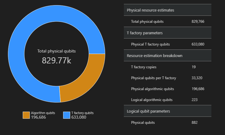
공간 다이어그램

알고리즘 및 T 팩터리에 사용되는 실제 큐비트의 분포는 알고리즘 디자인에 영향을 미칠 수 있는 요소입니다. 패키지를 사용하여 qsharp-widgets 이 분포를 시각화하여 알고리즘의 예상 공간 요구 사항을 더 잘 이해할 수 있습니다.

from qsharp_widgets import SpaceChart
SpaceChart(result)

이 예제에서는 알고리즘을 실행하는 데 필요한 실제 큐비트 수가 829766 196686 알고리즘 큐비트이고 그 중 633080은 T 팩터리 큐비트입니다.

Screenshot showing the space diagram of the Resource Estimator.

다양한 큐비트 기술에 대한 리소스 추정치 비교

Azure Quantum Resource Estimator를 사용하면 대상 매개 변수의 여러 구성을 실행하고 결과를 비교할 수 있습니다. 이는 다양한 큐비트 모델, QEC 스키마 또는 오류 예산의 비용을 비교하려는 경우에 유용합니다.

개체를 사용하여 추정 매개 변수 목록을 생성할 EstimatorParams 수도 있습니다.

from qsharp.estimator import EstimatorParams, QubitParams, QECScheme, LogicalCounts

labels = ["Gate-based µs, 10⁻³", "Gate-based µs, 10⁻⁴", "Gate-based ns, 10⁻³", "Gate-based ns, 10⁻⁴", "Majorana ns, 10⁻⁴", "Majorana ns, 10⁻⁶"]

params = EstimatorParams(6)
params.error_budget = 0.333
params.items[0].qubit_params.name = QubitParams.GATE_US_E3
params.items[1].qubit_params.name = QubitParams.GATE_US_E4
params.items[2].qubit_params.name = QubitParams.GATE_NS_E3
params.items[3].qubit_params.name = QubitParams.GATE_NS_E4
params.items[4].qubit_params.name = QubitParams.MAJ_NS_E4
params.items[4].qec_scheme.name = QECScheme.FLOQUET_CODE
params.items[5].qubit_params.name = QubitParams.MAJ_NS_E6
params.items[5].qec_scheme.name = QECScheme.FLOQUET_CODE

qsharp.estimate("RunProgram()", params=params).summary_data_frame(labels=labels)

큐비트 모델	논리 큐비트	논리 깊이	T 상태	코드 거리	T 팩터리	T 팩터리 분수	물리적 큐비트	rQOPS	물리적 런타임
게이트 기반 μs, 10⁻5	223 3.64M	4.70M	17	13	40.54 %	216.77k	21.86k	10시간
게이트 기반 µs, 10⁻⁴	223	3.64M	4.70M	9	14	43.17 %	63.57k	41.30k	5시간
게이트 기반 ns, 10⁻³	223 3.64M	4.70M	17	16	69.08 %	416.89k	32.79M	25초
게이트 기반 ns, 10⁻⁴	223 3.64M	4.70M	9	14	43.17 %	63.57k	61.94M	13초
Majorana ns, 10⁻⁴	223 3.64M	4.70M	9	19	82.75 %	501.48k	82.59M	10초
Majorana ns, 10⁻⁶	223 3.64M	4.70M	5	13	31.47 %	42.96k	148.67M	5초

논리 리소스 수에서 리소스 예측 추출

작업에 대한 몇 가지 예측을 이미 알고 있는 경우 리소스 예측 도구를 사용하면 알려진 예측을 프로그램의 전체 비용에 통합하여 실행 시간을 줄일 수 있습니다. 클래스를 LogicalCounts 사용하여 미리 계산된 리소스 예측 값에서 논리 리소스 추정값을 추출할 수 있습니다.

코드를 선택하여 새 셀을 추가한 다음, 다음 코드를 입력하고 실행합니다.

logical_counts = LogicalCounts({
    'numQubits': 12581,
    'tCount': 12,
    'rotationCount': 12,
    'rotationDepth': 12,
    'cczCount': 3731607428,
    'measurementCount': 1078154040})

logical_counts.estimate(params).summary_data_frame(labels=labels)

큐비트 모델	논리 큐비트	논리 깊이	T 상태	코드 거리	T 팩터리	T 팩터리 분수	물리적 큐비트	물리적 런타임
게이트 기반 μs, 10⁻5	25481	1.2e+10	1.5e+10	27	13	0.6%	37.38M	6년
게이트 기반 µs, 10⁻⁴	25481	1.2e+10	1.5e+10	13	14	0.8%	8.68M	3년
게이트 기반 ns, 10⁻³	25481	1.2e+10	1.5e+10	27	15	1.3%	37.65M	2일
게이트 기반 ns, 10⁻⁴	25481	1.2e+10	1.5e+10	13	18	1.2%	8.72M	18시간
Majorana ns, 10⁻⁴	25481	1.2e+10	1.5e+10	15	15	1.3%	26.11M	15시간
Majorana ns, 10⁻⁶	25481	1.2e+10	1.5e+10	7	13	0.5%	6.25M	7시간

결론

최악의 시나리오에서는 게이트 기반 μs 큐비트(초전도 큐비트와 같은 나노초 정권에서 작업 시간이 있는 큐비트)를 사용하는 양자 컴퓨터와 표면 QEC 코드는 Shor 알고리즘을 사용하여 2,048비트 정수의 계수가 되도록 6년 및 3738만 큐비트가 필요합니다.

게이트 기반 ns 이온 큐비트 및 동일한 surface 코드와 같은 다른 큐비트 기술을 사용하는 경우 큐비트 수는 크게 변하지 않지만 런타임은 최악의 경우에는 2일, 낙관적인 경우에는 18시간이 됩니다. 예를 들어 Majorana 기반 큐비트를 사용하여 큐비트 기술과 QEC 코드를 변경하는 경우 Shor 알고리즘을 사용하여 2048비트 정수를 인수분해하면 최상의 시나리오에서 625만 큐비트의 배열로 몇 시간 안에 완료할 수 있습니다.

실험에서 Majorana 큐비트와 Floquet QEC 코드를 사용하는 것이 Shor 알고리즘을 실행하고 2,048비트 정수로 계산하는 가장 좋은 선택이라고 결론을 내릴 수 있습니다.

계속

연습 - 실제 문제에 대한 리소스 예측

Shor 알고리즘 작성

Shor 알고리즘 예측

공간 다이어그램

다양한 큐비트 기술에 대한 리소스 추정치 비교

논리 리소스 수에서 리소스 예측 추출

결론

피드백