Lakehouse tutorial: Prepare and transform data in the lakehouse

In this tutorial, you use notebooks with Spark runtime to transform and prepare raw data in your lakehouse.

Prerequisites

Before you begin, you must complete the previous tutorials in this series:

1. Create a lakehouse
2. Ingest data into the lakehouse
3. Ensure lakehouse schemas are enabled in your lakehouse.

Prepare data

From the previous tutorial steps, you have raw data ingested from the source to the Files section of the lakehouse. Now you can transform that data and prepare it for creating Delta tables.

1. Download the notebooks from the Lakehouse Tutorial Source Code folder.

2. In your browser, go to your Fabric workspace in the Fabric portal.

3. Select Import > Notebook > From this computer.

   

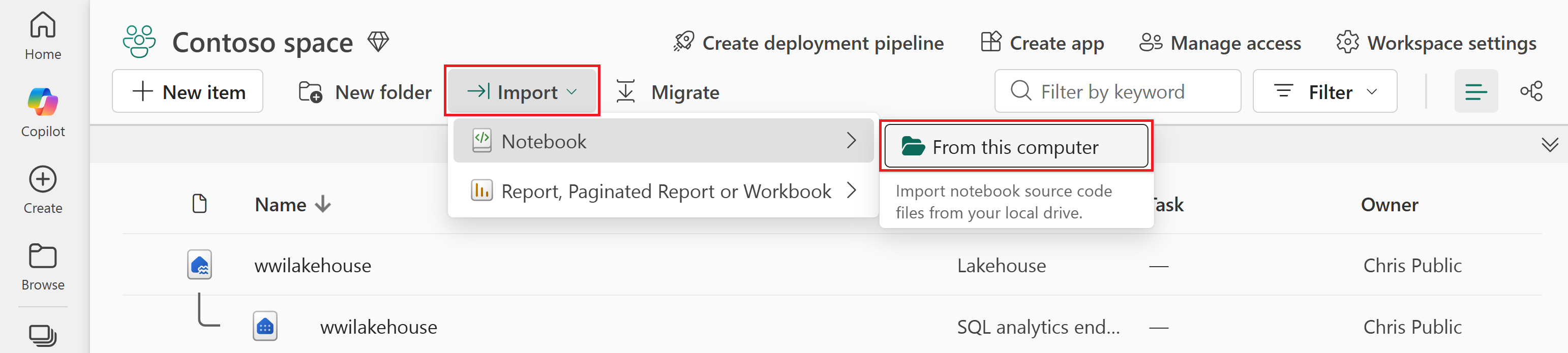
4. Select Upload from the Import status pane that opens on the right side of the screen.

5. Select only the notebook that matches your preferred coding language.

   • PySpark (Prepare and transform data - PySpark.ipynb)
   • Spark SQL (Prepare and transform data - Spark SQL.ipynb)

6. Select Open. A notification indicating the status of the import appears in the top right corner of the browser window.

7. After the import is successful, go to the items view of the workspace to verify the imported notebook.

   

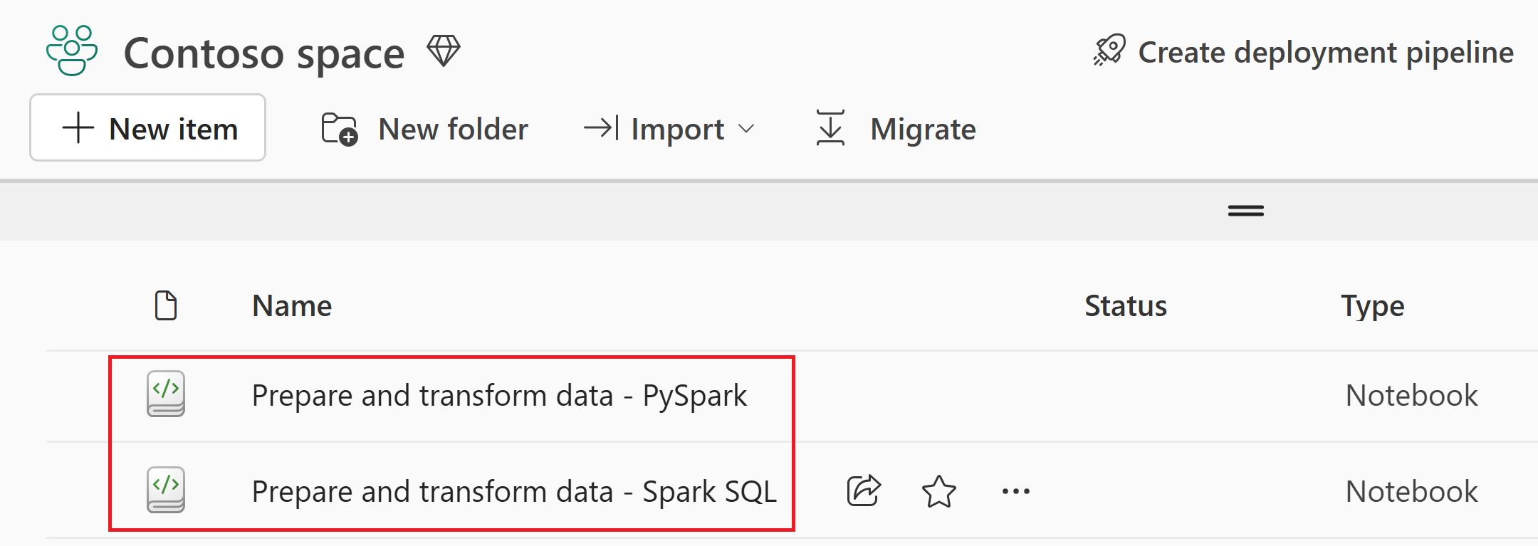
8. Select the wwilakehouse lakehouse to open it, so that the notebook you open next is linked to it.

9. From the top navigation menu, select Open notebook > Existing notebook.

   

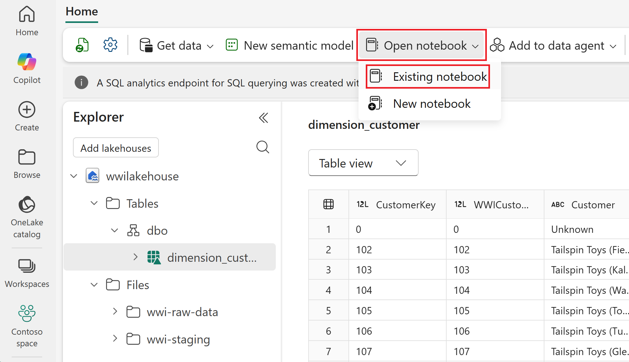
10. Select your imported notebook for PySpark or Spark SQL and select Open. The notebook is already linked to your opened lakehouse, as shown in the lakehouse Explorer.

You're now ready to run the notebook cells that create and transform your Delta tables.

In the following sections, run the notebook cells sequentially. To execute a cell, select the Run icon that appears to the left of the cell on hover. You can also select Run all on the top ribbon (Home) to run all cells in sequence.

Important

This tutorial requires lakehouse schemas to be enabled. If schemas aren't enabled, the code in this tutorial won't work as intended.

In the imported notebook, you see both Path 1 and Path 2 sections. For this tutorial, use Path 1 (lakehouse schemas enabled) and ignore Path 2 (lakehouse schemas not enabled).

Create Delta tables

In this section, you run the notebook cells to create Delta tables from the raw data.

The tables follow a star schema, which is a common pattern for organizing analytical data:

• A fact table (fact_sale) contains the measurable events of the business — in this case, individual sales transactions with quantities, prices, and profit.
• Dimension tables (dimension_city, dimension_customer, dimension_date, dimension_employee, dimension_stock_item) contain the descriptive attributes that give context to the facts, such as where a sale happened, who made it, and when.

In this tutorial page, select the tab that matches the notebook you imported, and keep using that same tab for all steps. The tabs are in this article, not in the notebook.

1. Cell 1 - Spark session configuration. This cell enables two Fabric features that optimize how data is written and read in subsequent cells. V-order optimizes the parquet file layout for faster reads and better compression. Optimize write reduces the number of files written and increases individual file size.

   Run this cell, and wait for it to finish before moving on to the next step.

   PySpark

   spark.conf.set("spark.sql.parquet.vorder.enabled", "true")
   spark.conf.set("spark.microsoft.delta.optimizeWrite.enabled", "true")
   spark.conf.set("spark.microsoft.delta.optimizeWrite.binSize", "1073741824")
   

   Spark SQL

   %%sql
   SET spark.sql.parquet.vorder.enabled=true;
   SET spark.microsoft.delta.optimizeWrite.enabled=true;
   SET spark.microsoft.delta.optimizeWrite.binSize=1073741824;
   

   Tip

   You don't need to specify any Spark pool or cluster details. Fabric provides a default Spark pool called Live Pool for every workspace. When you execute the first cell, the live pool starts in a few seconds and establishes the Spark session. Subsequent cells run almost instantaneously while the session is active.

2. Cell 2 - Fact - Sale. This cell reads raw parquet data from Files/wwi-raw-data/full/fact_sale_1y_full, adds date part columns (Year, Quarter, and Month), and writes fact_sale as a Delta table partitioned by Year and Quarter.

   Run this cell, and wait for it to finish before moving on to the next step.

   PySpark

   from pyspark.sql.functions import col, year, month, quarter
   
   table_name = 'fact_sale'
   
   df = spark.read.format("parquet").load('Files/wwi-raw-data/full/fact_sale_1y_full')
   df = df.withColumn('Year', year(col("InvoiceDateKey")))
   df = df.withColumn('Quarter', quarter(col("InvoiceDateKey")))
   df = df.withColumn('Month', month(col("InvoiceDateKey")))
   
   df.write.mode("overwrite").format("delta").partitionBy("Year","Quarter").save("Tables/dbo/" + table_name)
   

   Spark SQL

   %%sql
   CREATE OR REPLACE TABLE delta.`Tables/dbo/fact_sale`
   USING DELTA
   PARTITIONED BY (Year, Quarter)
   AS
   SELECT
      *,
      year(InvoiceDateKey) AS Year,
      quarter(InvoiceDateKey) AS Quarter,
      month(InvoiceDateKey) AS Month
   FROM parquet.`Files/wwi-raw-data/full/fact_sale_1y_full`;
   

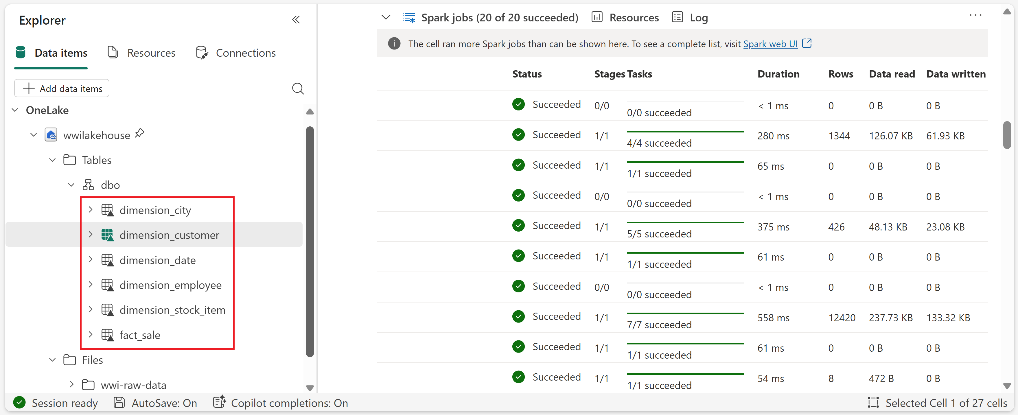
3. Cell 3 - Dimensions. This cell reads the five dimension parquet datasets and writes them as Delta tables (dimension_city, dimension_customer, dimension_date, dimension_employee, and dimension_stock_item) under Tables/dbo/....

   Run this cell, and wait for it to finish before moving on to the next step.

   PySpark

   def loadFullDataFromSource(table_name):
      df = spark.read.format("parquet").load('Files/wwi-raw-data/full/' + table_name)
      df = df.drop("Photo")
      df.write.mode("overwrite").format("delta").save("Tables/dbo/" + table_name)
   
   full_tables = [
      'dimension_city',
      'dimension_customer',
      'dimension_date',
      'dimension_employee',
      'dimension_stock_item'
   ]
   
   for table in full_tables:
      loadFullDataFromSource(table)
   

   Spark SQL

   %%sql
   CREATE OR REPLACE TABLE delta.`Tables/dbo/dimension_city` USING DELTA AS SELECT * FROM parquet.`Files/wwi-raw-data/full/dimension_city`;
   CREATE OR REPLACE TABLE delta.`Tables/dbo/dimension_customer` USING DELTA AS SELECT * FROM parquet.`Files/wwi-raw-data/full/dimension_customer`;
   CREATE OR REPLACE TABLE delta.`Tables/dbo/dimension_date` USING DELTA AS SELECT * FROM parquet.`Files/wwi-raw-data/full/dimension_date`;
   CREATE OR REPLACE TABLE delta.`Tables/dbo/dimension_employee` USING DELTA AS SELECT * FROM parquet.`Files/wwi-raw-data/full/dimension_employee`;
   CREATE OR REPLACE TABLE delta.`Tables/dbo/dimension_stock_item` USING DELTA AS SELECT * FROM parquet.`Files/wwi-raw-data/full/dimension_stock_item`;
   

4. To validate the created tables, right-click the wwilakehouse lakehouse in the explorer and then select Refresh. The tables appear.

   

Transform data for business aggregates

In this section, you continue in the same notebook and run the next cells to create aggregate tables from the Delta tables you created in the previous section.

1. Make sure the notebook is still linked to wwilakehouse.

2. Cell 4 - Load source tables for transformation (PySpark only). If you're using the PySpark notebook, run this cell to load Delta tables into DataFrames for the aggregation steps that follow.

   Run this cell, and wait for it to finish before moving on to the next step.

   PySpark

   df_fact_sale = spark.read.format("delta").load("Tables/dbo/fact_sale")
   df_dimension_date = spark.read.format("delta").load("Tables/dbo/dimension_date")
   df_dimension_city = spark.read.format("delta").load("Tables/dbo/dimension_city")
   

   Spark SQL

   No action is required for Spark SQL in this step.

3. Cell 5 - Create aggregate_sale_by_date_city. This cell joins sales, date, and city data, then creates the city-level aggregate table.

   Run this cell, and wait for it to finish before moving on to the next step.

   PySpark

   sale_by_date_city = (
      df_fact_sale.alias("sale")
      .join(df_dimension_date.alias("date"), df_fact_sale.InvoiceDateKey == df_dimension_date.Date, "inner")
      .join(df_dimension_city.alias("city"), df_fact_sale.CityKey == df_dimension_city.CityKey, "inner")
      .select("date.Date", "date.CalendarMonthLabel", "date.Day", "date.ShortMonth", "date.CalendarYear", "city.City", "city.StateProvince", "city.SalesTerritory", "sale.TotalExcludingTax", "sale.TaxAmount", "sale.TotalIncludingTax", "sale.Profit")
      .groupBy("date.Date", "date.CalendarMonthLabel", "date.Day", "date.ShortMonth", "date.CalendarYear", "city.City", "city.StateProvince", "city.SalesTerritory")
      .sum("sale.TotalExcludingTax", "sale.TaxAmount", "sale.TotalIncludingTax", "sale.Profit")
      .withColumnRenamed("sum(TotalExcludingTax)", "SumOfTotalExcludingTax")
      .withColumnRenamed("sum(TaxAmount)", "SumOfTaxAmount")
      .withColumnRenamed("sum(TotalIncludingTax)", "SumOfTotalIncludingTax")
      .withColumnRenamed("sum(Profit)", "SumOfProfit")
      .orderBy("date.Date", "city.StateProvince", "city.City")
   )
   
   sale_by_date_city.write.mode("overwrite").format("delta").option("overwriteSchema", "true").save("Tables/dbo/aggregate_sale_by_date_city")
   

   Spark SQL

   %%sql
   CREATE OR REPLACE TEMPORARY VIEW sale_by_date_city
   AS
   SELECT
         DD.Date, DD.CalendarMonthLabel
         , DD.Day, DD.ShortMonth Month, CalendarYear Year
         , DC.City, DC.StateProvince, DC.SalesTerritory
         , SUM(FS.TotalExcludingTax) SumOfTotalExcludingTax
         , SUM(FS.TaxAmount) SumOfTaxAmount
         , SUM(FS.TotalIncludingTax) SumOfTotalIncludingTax
         , SUM(FS.Profit) SumOfProfit
   FROM delta.`Tables/dbo/fact_sale` FS
   INNER JOIN delta.`Tables/dbo/dimension_date` DD ON FS.InvoiceDateKey = DD.Date
   INNER JOIN delta.`Tables/dbo/dimension_city` DC ON FS.CityKey = DC.CityKey
   GROUP BY DD.Date, DD.CalendarMonthLabel, DD.Day, DD.ShortMonth, DD.CalendarYear, DC.City, DC.StateProvince, DC.SalesTerritory
   ORDER BY DD.Date ASC, DC.StateProvince ASC, DC.City ASC;
   
   CREATE OR REPLACE TABLE delta.`Tables/dbo/aggregate_sale_by_date_city`
   AS
   SELECT * FROM sale_by_date_city;
   

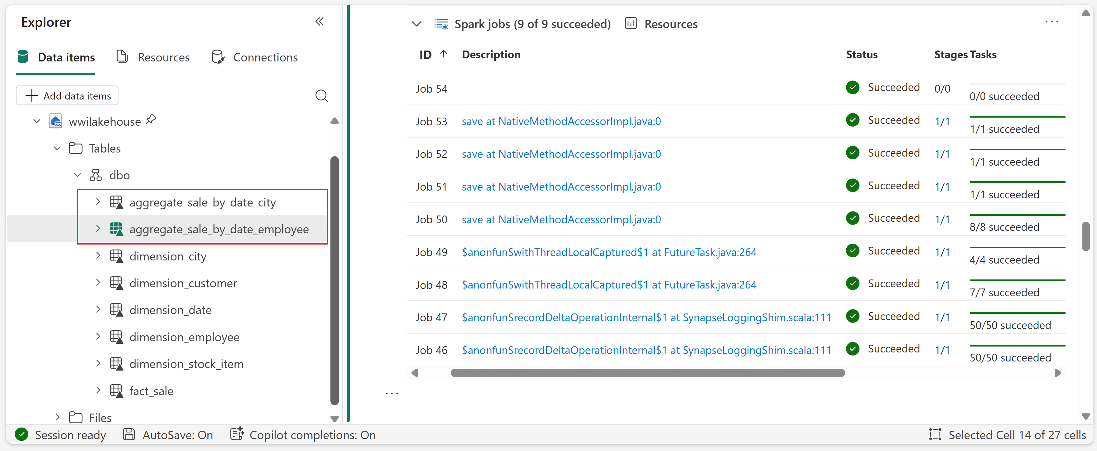
4. Cell 6 - Create aggregate_sale_by_date_employee. This cell joins sales, date, and employee data, then creates the employee-level aggregate table.

   Run this cell, and wait for it to finish before moving on to the next step.

   PySpark

   spark.sql("""
   CREATE OR REPLACE TEMPORARY VIEW sale_by_date_employee
   AS
   SELECT
              DD.Date, DD.CalendarMonthLabel
           , DD.Day, DD.ShortMonth Month, CalendarYear Year
           , DE.PreferredName, DE.Employee
           , SUM(FS.TotalExcludingTax) SumOfTotalExcludingTax
           , SUM(FS.TaxAmount) SumOfTaxAmount
           , SUM(FS.TotalIncludingTax) SumOfTotalIncludingTax
           , SUM(FS.Profit) SumOfProfit
   FROM delta.`Tables/dbo/fact_sale` FS
   INNER JOIN delta.`Tables/dbo/dimension_date` DD ON FS.InvoiceDateKey = DD.Date
   INNER JOIN delta.`Tables/dbo/dimension_employee` DE ON FS.SalespersonKey = DE.EmployeeKey
   GROUP BY DD.Date, DD.CalendarMonthLabel, DD.Day, DD.ShortMonth, DD.CalendarYear, DE.PreferredName, DE.Employee
   ORDER BY DD.Date ASC, DE.PreferredName ASC, DE.Employee ASC
   """)
   
   sale_by_date_employee = spark.sql("SELECT * FROM sale_by_date_employee")
   sale_by_date_employee.write.mode("overwrite").format("delta").option("overwriteSchema", "true").save("Tables/dbo/aggregate_sale_by_date_employee")
   

   Spark SQL

   %%sql
   CREATE OR REPLACE TEMPORARY VIEW sale_by_date_employee
   AS
   SELECT
              DD.Date, DD.CalendarMonthLabel
           , DD.Day, DD.ShortMonth Month, CalendarYear Year
           , DE.PreferredName, DE.Employee
           , SUM(FS.TotalExcludingTax) SumOfTotalExcludingTax
           , SUM(FS.TaxAmount) SumOfTaxAmount
           , SUM(FS.TotalIncludingTax) SumOfTotalIncludingTax
           , SUM(FS.Profit) SumOfProfit
   FROM delta.`Tables/dbo/fact_sale` FS
   INNER JOIN delta.`Tables/dbo/dimension_date` DD ON FS.InvoiceDateKey = DD.Date
   INNER JOIN delta.`Tables/dbo/dimension_employee` DE ON FS.SalespersonKey = DE.EmployeeKey
   GROUP BY DD.Date, DD.CalendarMonthLabel, DD.Day, DD.ShortMonth, DD.CalendarYear, DE.PreferredName, DE.Employee
   ORDER BY DD.Date ASC, DE.PreferredName ASC, DE.Employee ASC;
   
   CREATE OR REPLACE TABLE delta.`Tables/dbo/aggregate_sale_by_date_employee`
   AS
   SELECT * FROM sale_by_date_employee;
   

5. To validate the created tables, right-click the wwilakehouse lakehouse in the explorer and then select Refresh. The aggregate tables appear.

   

This tutorial writes data as Delta lake files. Fabric automatically discovers and registers these tables in the metastore, so you don't need to run separate CREATE TABLE statements.

Next step

Create a semantic model and build a report