Pivot columns

In Power Query, you can create a table that contains an aggregate value for each unique value in a column. Power Query groups each unique value, does an aggregate calculation for each value, and pivots the column into a new table.

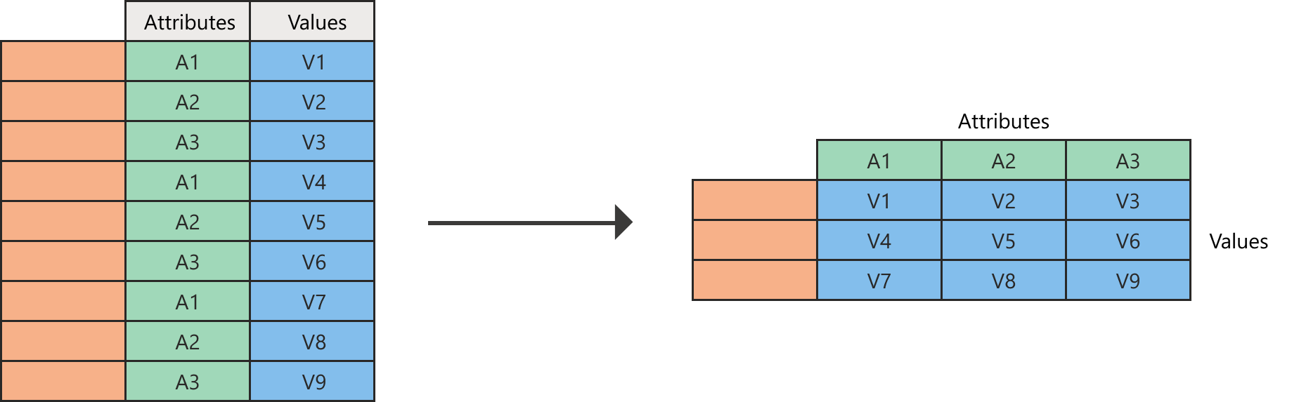
Diagram showing a table on the left with a blank column and rows. An Attributes column contains nine rows with A1, A2, and A3 repeated three times. A Values column contains, from top to bottom, values V1 through V9. With the columns pivoted, a table on the right contains a blank column and rows, the Attributes values A1, A2, and A3 as column headers, with the A1 column containing the values V1, V4, and V7, the A2 column containing the values V2, V5, and V8, and the A3 column containing the values V3, V6, and V9.

Imagine a table like the one in the following image.

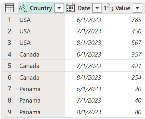
Table containing a Country column set as the Text data type, a Date column set as the Data data type, and a Value column set as the Whole number data type. The Country column contains USA in the first three rows, Canada in the next three rows, and Panama in the last three rows. The Date column contains 6/1/2020 in the first, forth, and seventh rows, 7/1/2020 in the second, fifth, and eighth rows, and 8/1/2020 in the third, sixth, and ninth rows.

This table contains values by country and date in a simple table. In this example, you want to transform this table into the one where the date column is pivoted, as shown in the following image.

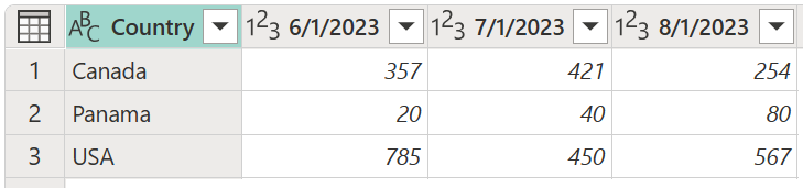
Table containing a Country column set in the Text data type, and 6/1/2020, 7/1/2020, and 8/1/2020 columns set as the Whole number data type. The Country column contains Canada in row 1, Panama in row 2, and USA in row 3.

Note

During the pivot columns operation, Power Query will sort the table based on the values found on the first column—at the left side of the table—in ascending order.

To pivot a column

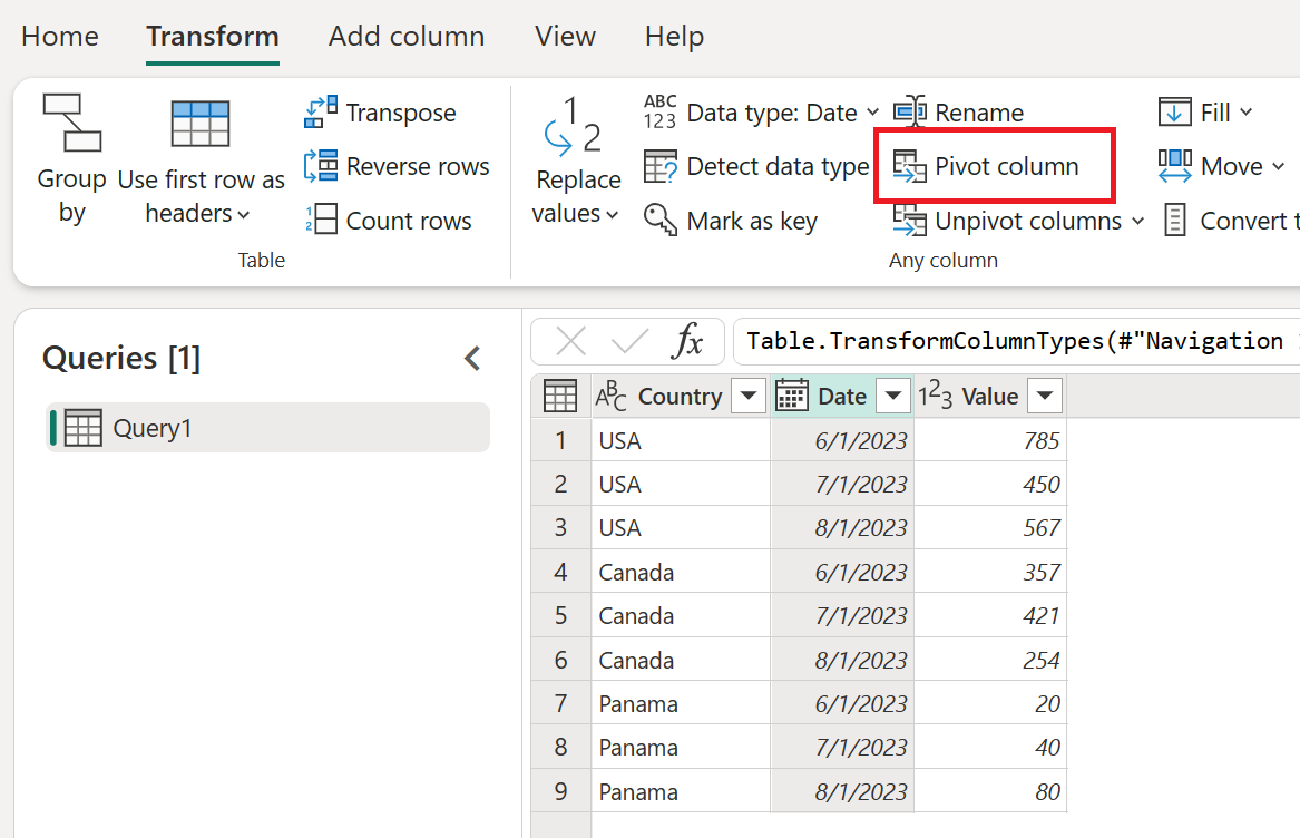
1. Select the column that you want to pivot.

2. On the Transform tab in the Any column group, select Pivot column.

   

3. In the Pivot column dialog box, in the Value column list, select Value.

   

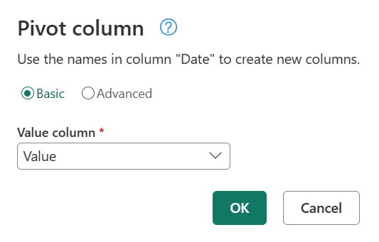
   By default, Power Query will try to do a sum as the aggregation, but you can select the Advanced option to see other available aggregations.

   

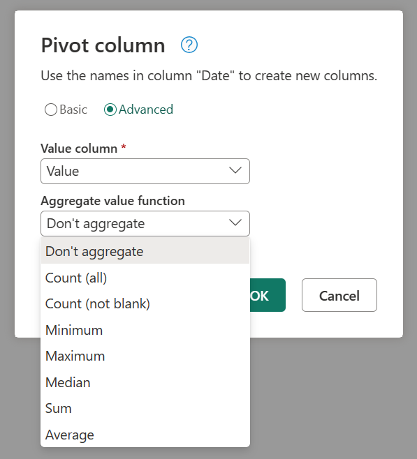
The available options are:

• Don't aggregate
• Count (all)
• Count (not blank)
• Minimum
• Maximum
• Median
• Sum
• Average

Pivoting columns that can't be aggregated

You can pivot columns without aggregating when you're working with columns that can't be aggregated, or aggregation isn't required for what you're trying to do. For example, imagine a table like the following image, that has Country, Position, and Product as fields.

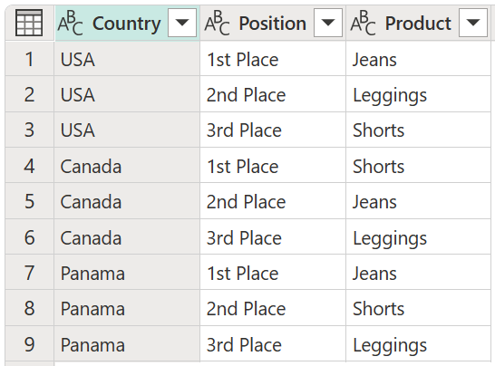
Table with Country column containing USA in the first three rows, Canada in the next three rows, and Panama in the last three rows. The Position column contains First Place in the first, fourth, and seventh rows, Second Place in the second, fifth, and eighth rows, and third Place in the third, sixth, and ninth rows.

Let's say you want to pivot the Position column in this table so you can have its values as new columns. For the values of these new columns, you'll use the values from the Product column. Select the Position column, and then select Pivot column to pivot that column.

In the Pivot column dialog box, select the Product column as the value column. Select the Advanced option button in the Pivot columns dialog box, and then select Don't aggregate.

The result of this operation will yield the result shown in the following image.

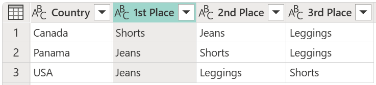
Table containing Country, First Place, second Place, and Third Place columns, with the Country column containing Canada in row 1, Panama in row 2, and USA in row 3.

Errors when using the Don't aggregate option

The way the Don't aggregate option works is that it grabs a single value for the pivot operation to be placed as the value for the intersection of the column and row pair. For example, let's say you have a table like the one in the following image.

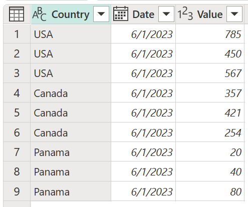
Table with a Country, Date, and Value columns. The Country column contains USA in the first three rows, Canada in the next three rows, and Panama in the last three rows. The Date column contains a date of 6/1/2020 in all rows. The value column contains various whole numbers between 20 and 785.

You want to pivot that table by using the Date column, and you want to use the values from the Value column. Because this pivot would make your table have just the Country values on rows and the Dates as columns, you'd get an error for every single cell value because there are multiple rows for every combination of Country and Date. The outcome of the Pivot column operation will yield the results shown in the following image.

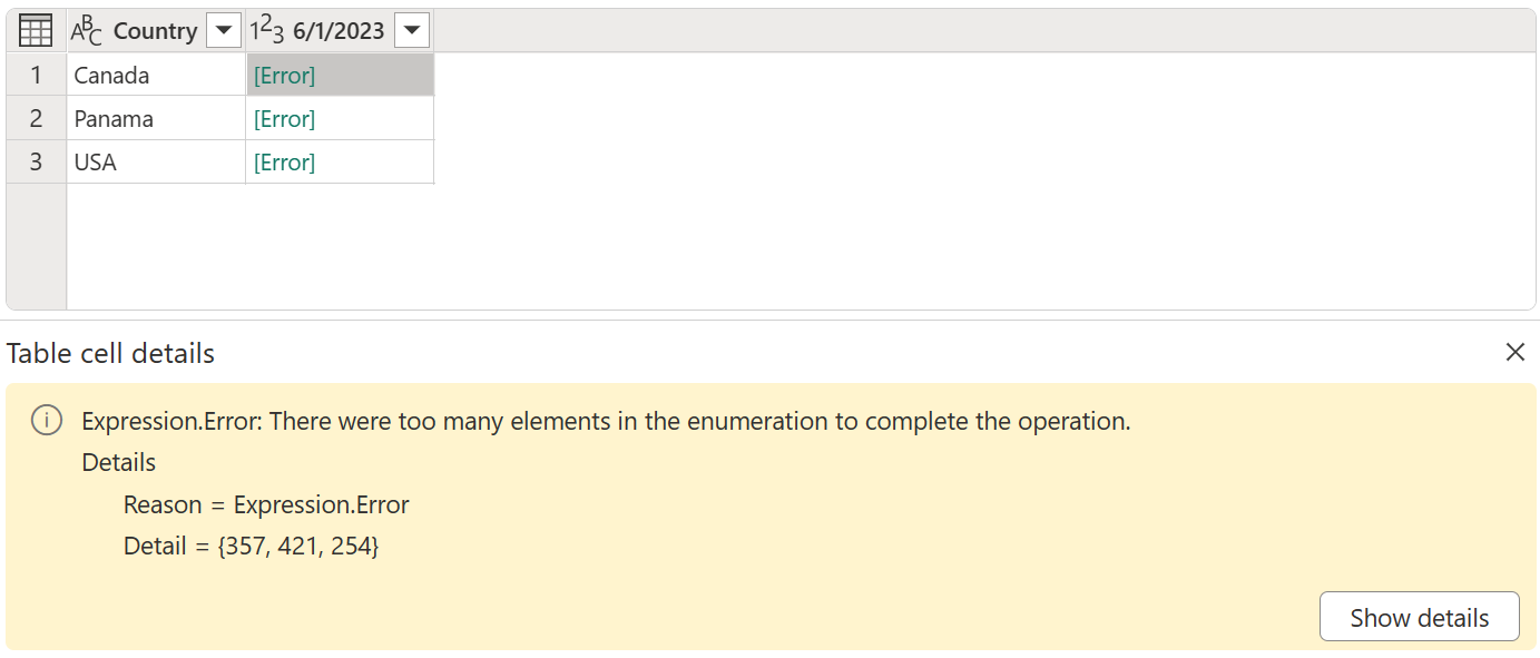
Power Query Editor pane showing a table with Country and 6/1/2020 columns. The Country column contains Canada in the first row, Panama in the second row, and USA in the third row. All of the rows under the 6/1/2020 column contain Errors. Under the table is another pane that shows the expression error with the "There are too many elements in the enumeration to complete the operation" message.

Notice the error message "Expression.Error: There were too many elements in the enumeration to complete the operation." This error occurs because the Don't aggregate operation only expects a single value for the country and date combination.