GQL language guide for graph in Microsoft Fabric

GQL (Graph Query Language) is the ISO-standardized query language for graph databases. Use GQL to query, analyze, and work with graph data efficiently with graph in Microsoft Fabric.

The same ISO working group that standardizes SQL develops GQL. As a result, GQL shares many concepts with SQL, including expressions, predicates, and data types. If you have SQL experience, you can apply much of that knowledge to GQL.

This article is the end-to-end guide to GQL in graph. It explains how the language fits together and links to focused references for complete syntax and type details. It covers:

• Core concepts: Graph data structures, patterns, and query fundamentals
• Essential statements: MATCH, FILTER, LET, WHEN, ORDER BY, LIMIT, and RETURN
• Data types and expressions: Value types, operators, and built-in functions
• Advanced techniques: Multi-statement composition, variable scoping, and aggregation strategies

Note

The official International Standard for GQL is ISO/IEC 39075 Information Technology - Database Languages - GQL.

If you're looking for task-oriented guidance instead of a language walkthrough, see the how-to guides:

• Write common GQL queries — neighbors, multi-hop traversal, shared connections, and entity existence checks
• Filter and aggregate graph data — FILTER, WHERE, GROUP BY, and aggregate functions
• Write graph pattern queries — multi-hop patterns, path modes, variable reuse, and OPTIONAL MATCH
• Optimize GQL query performance — filtering strategy, traversal limits, and key constraint recommendations

Use the focused reference articles when you need complete details:

Information needed	Definitive article
Syntax at a glance	GQL quick reference
Node, edge, path, and pattern composition syntax	GQL graph patterns
Operators, predicates, and functions	GQL expressions, predicates, and functions
Literal syntax, value behavior, and type conversions	GQL values and value types
Graph type definitions and constraints	GQL graph types
Current ISO GQL feature coverage	GQL standard conformance
Current Fabric-specific restrictions and limits	Current limitations

Prerequisites

Before you start, make sure you're familiar with these concepts:

• Basic understanding of databases - Experience with any database system such as relational (SQL), NoSQL, or graph is helpful.
• Graph concepts - Understanding of nodes, edges, and relationships in connected data.
• Query fundamentals - Knowledge of basic query concepts like filtering, sorting, and aggregation.

Recommended background:

• Experience with SQL or openCypher languages makes learning GQL syntax easier (they're GQL's roots).
• Familiarity with data modeling helps with graph schema design.
• Understanding of your specific use case for graph data.

What you need:

• Access to a graph workspace with query capabilities.
• Sample data or willingness to work with our social network examples.
• Basic text editor for writing queries.

Tip

If you're new to graph databases, start with the graph data models overview before continuing with this guide.

What makes GQL special

GQL is designed specifically for graph data, so its syntax directly expresses how entities are connected. Where SQL commonly expresses relationships through joins between tables, GQL uses graph patterns that resemble diagrams of the data.

For example, the following query finds pairs of people who know each other and were both born before 1999:

MATCH (person:Person)-[:knows]-(friend:Person)
WHERE person.birthday < 19990101
  AND friend.birthday < 19990101
RETURN person.firstName || ' ' || person.lastName AS person_name,
       friend.firstName || ' ' || friend.lastName AS friend_name

The pattern (person:Person)-[:knows]-(friend:Person) shows the relationship structure to match. Variables bind the two people so the query can filter and return their properties.

GQL fundamentals

These concepts form the foundation of GQL:

• Graphs contain nodes and edges with labels and properties.
• Graph types formally define the node types, edge types, and constraints permitted in a graph.
• Queries use statements such as MATCH, FILTER, and RETURN to process data and produce results.
• Patterns describe the graph structures to match.
• Expressions calculate, transform, and compare values.
• Predicates are Boolean expressions used to test conditions.
• Value types define the kinds of values that queries can process and graph properties can store.

Understand graph data

To work with GQL, you need to understand the labeled property graph structure that the language queries.

Nodes and edges: the building blocks

A labeled property graph contains two kinds of graph elements:

• Nodes typically represent entities, such as people, organizations, posts, or products.
• Edges represent connections between nodes, such as a person knowing another person or working at a company.

Every graph element has an internal identity, one or more labels, and a set of properties. Labels classify elements, such as Person or knows. Properties are name-value pairs, such as firstName: 'Alice' or birthday: 19730108u. In Graph, an edge always has exactly one label.

Each edge connects exactly two nodes: an origin and a target. Edge direction is part of the graph structure. For example, a workAt edge can connect a Person origin to a Company target.

Note

Graph currently doesn't support creating undirected edges. You can query an existing directed edge in either direction by using an any-directed edge pattern such as -[:knows]-.

Graphs are well-formed: every edge connects two nodes that exist in the same graph.

Graph models and graph types

A Fabric graph model defines the node types, edge types, properties, source mappings, and keys available in a graph. It specifies which source-table rows become nodes and edges and how those elements connect. For modeling guidance, see Design a graph schema.

The GQL standard uses a graph type to formally describe permitted node types, edge types, properties, and constraints. Graph types are the language-level counterpart to the structure represented by a Fabric graph model, but Graph doesn't currently accept GQL graph-type declarations directly. For the formal syntax and concepts, see GQL graph types.

Example graph used in this guide

Examples use the social network sample dataset, which includes people, places, organizations, messages, tags, and the edges that connect them.

The sample graph connects these areas:

• People know other people, work at companies, and study at universities.
• Cities, countries or regions, and continents form a geographic hierarchy.
• Forums contain posts, and people create posts and comments.
• Tags categorize content and represent people's interests.

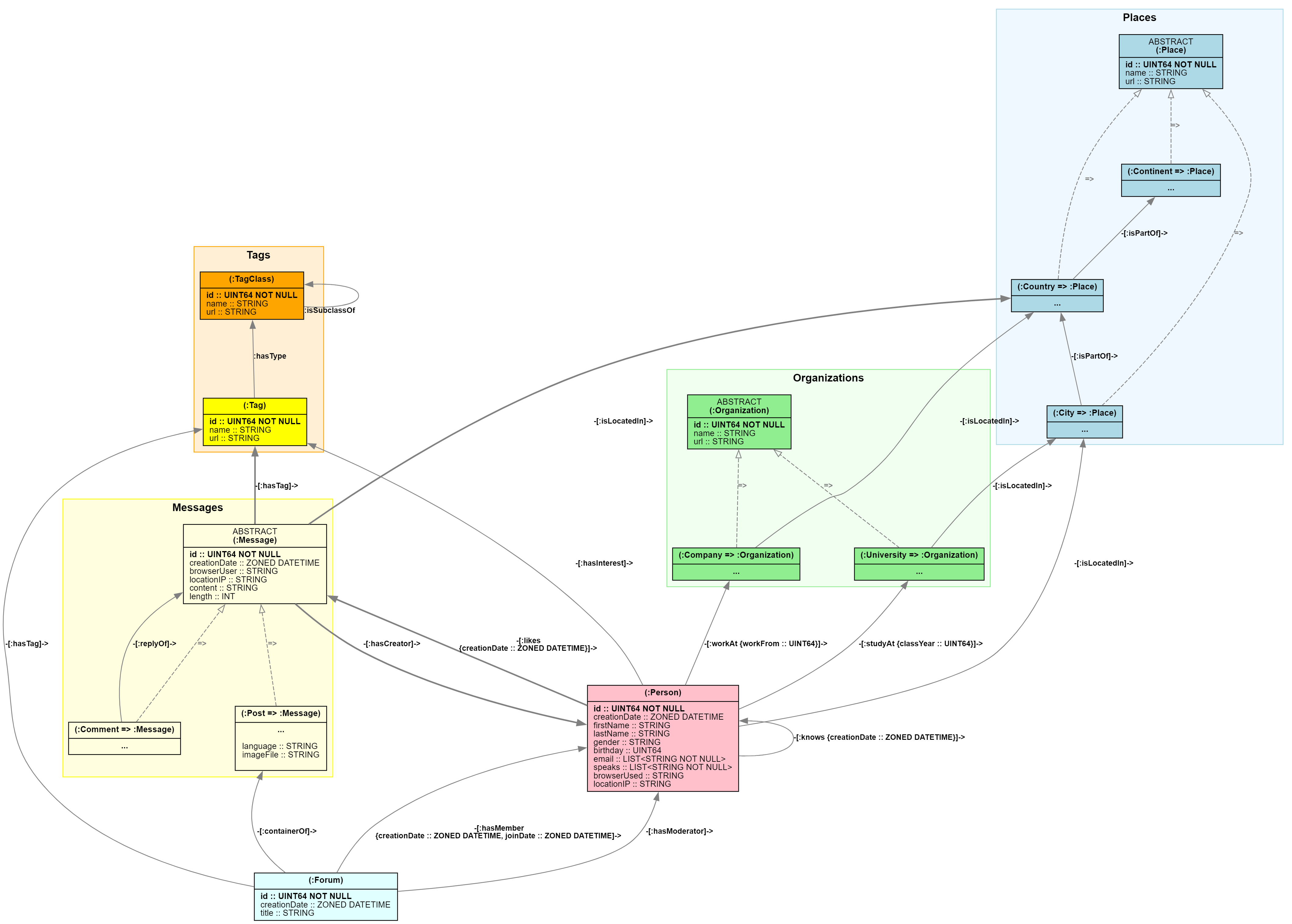
For the complete example structure, see the social network schema example. For general graph concepts, see Labeled property graphs.

Your first GQL queries

Now that you understand graph basics, let's see how to query graph data using GQL. These examples build from simple to complex, showing you how GQL's approach makes graph queries intuitive and powerful.

Start simple: find all people

Begin with the most basic query possible. Find the names (first name, last name) of all the people (:Persons) in the graph.

MATCH (p:Person)
RETURN p.firstName, p.lastName

This query runs as follows:

1. MATCH finds all nodes labeled Person.
2. RETURN shows their first and last names.

Add filtering: find specific people

Now find people with specific characteristics. In this case, find everyone named Alice and show their names and birthdays.

MATCH (p:Person)
FILTER p.firstName = 'Alice'
RETURN p.firstName, p.lastName, p.birthday

This query runs as follows:

1. MATCH finds all nodes (p) labeled Person.
2. FILTER nodes (p) whose first name is Alice.
3. RETURN shows their first, last name, and birthday.

Basic query structure

Basic GQL queries all follow a consistent pattern: a sequence of statements that work together to find, filter, and return data. Most queries start with MATCH to find patterns in the graph and end with RETURN to specify the output.

Here's a simple query that finds pairs of people who know each other and share the same birthday, then returns the total count of those friend pairs.

MATCH (n:Person)-[:knows]-(m:Person)
FILTER n.birthday = m.birthday
RETURN count(*) AS same_age_friends

This query runs as follows:

1. MATCH finds all pairs of Person nodes that know each other.
2. FILTER keeps only the pairs where both people have the same birthday.
3. RETURN counts how many such friend pairs exist.

Tip

You can also filter directly in a pattern by appending a WHERE clause. For example, MATCH (n:Person WHERE n.birthday < 19900101) matches only Person nodes with a birthday value before 1990.

GQL supports C-style // line comments, SQL-style -- line comments, and C-style /* */ block comments.

Common statements

• MATCH: Identifies the graph pattern to search for—this is where you define the structure of the data you're interested in.
• LET: Assigns new variables or computed values based on matched data—adds derived columns to the result.
• FOR: Expands a list into rows, with an optional zero-based offset or one-based ordinal position.
• CALL: Runs an inline subquery for each input row and adds the columns returned by the subquery.
• FILTER: Narrows down the results by applying conditions—removes rows that don’t meet the criteria.
• ORDER BY: Sorts the filtered data—helps organize the output based on one or more fields.
• OFFSET and LIMIT: Restrict the number of rows returned—useful for pagination or top-k queries.
• RETURN: Specifies the final output—defines what data should be included in the result set and performs aggregation.
• NEXT: Starts another query stage by using the columns returned from the previous stage.

How statements work together

GQL statements form a pipeline, where each statement processes the output of the previous one. This sequential execution makes queries easy to read and debug because the execution order matches the reading order.

Key points:

• Statements effectively execute sequentially.
• Each statement transforms data and passes it to the next.
• This process creates a clear, predictable data flow that simplifies complex queries.
• NEXT starts a new query stage. Only columns projected by the preceding RETURN statement are available in the next stage.
• UNION, UNION DISTINCT, and UNION ALL combine the results of complete query blocks.

Note

Statements have a defined logical order. Write queries according to this data flow rather than relying on a particular physical execution strategy.

Example of statement composition

The following GQL query finds the first 10 people working at companies with "Air" in their name, sorts them by full name, and returns their full name along with the name of their companies.

-- Data flows: Match → Let → Filter → Order → Limit → Return
MATCH (p:Person)-[:workAt]->(c:Company)           -- Input: unit table, Output: (p, c) table
LET fullName = p.firstName || ' ' || p.lastName   -- Input: (p, c) table, Output: (p, c, fullName) table
FILTER c.name CONTAINS 'Air'                      -- Input: (p, c, fullName) table, Output: filtered table
ORDER BY fullName                                 -- Input: filtered table, Output: sorted table
LIMIT 10                                          -- Input: sorted table, Output: top 10 rows table
RETURN fullName, c.name AS companyName            -- Input: top 10 rows table
                                                  -- Output: projected (fullName, companyName) result table

This query runs as follows:

1. MATCH finds people who work at companies.
2. LET creates full names by combining first and family names.
3. FILTER keeps only employees of companies with "Air" in their company name.
4. ORDER BY sorts by full name.
5. LIMIT takes the first 10 results.
6. RETURN returns full names and company names.

Variables connect your data

Variables, such as p, c, and fullName in the previous examples, carry data between statements. When you reuse a variable name, GQL automatically ensures it refers to the same data, creating powerful join conditions. Variables are sometimes also called binding variables.

You can categorize variables in different ways:

By binding source:

• Pattern variables - bound by matching graph patterns
• Regular variables - bound by other language constructs

Pattern variable types:

• Element variables - bind to graph element reference values
  • Node variables - bind to individual nodes
  • Edge variables - bind to individual edges
• Path variables - bind to path values representing matched paths

By reference degree:

• Singleton variables - bind to individual element reference values from patterns
• Group variables - bind to lists of element reference values from variable-length patterns. For details, see Aggregate functions.

Execution outcomes and results

When you run a query, you get back an execution outcome that consists of:

• A result, normally a result table with the data from your RETURN statement.
• Status information that shows whether the query succeeded or not.

Result tables

The result table - if present - is the actual result of query execution.

A result table includes information about the name and type of its columns, a preferred column name sequence to be used for displaying results, whether the table is ordered, and the actual rows themselves.

Note

If execution fails, no result table is included in the execution outcome.

Omitted results

GQL also defines an omitted result for statements that never produce rows, independent of the data or the evaluation outcome. An omitted result has successful-completion status code 00001.

An omitted result differs from an empty result table. An empty table means that a row-producing query was evaluated but produced no rows. The Query API can represent an omitted result with result kind NOTHING.

Graph reserves omitted results for future data definition language (DDL) and data manipulation language (DML) statement support. Current query statements produce table results, including empty tables.

Status information

During query execution, the process detects various noteworthy conditions, such as errors or warnings. Each condition is recorded by a status object in the status information of the execution outcome.

The status information consists of a primary status object and a (possibly empty) list of other status objects. The primary status object always exists and indicates whether query execution was successful or failed.

Every status object includes a five-character alphanumeric code and a description of the recorded condition.

The Query API uses the following primary status codes:

API status code	Meaning
00000	Successful completion with at least one row.
00001	Successful completion with an omitted result. Reserved for future DDL and DML support.
01000	A warning or informational condition.
02000	No rows are currently available from a row-producing query.
42000	A user-correctable query error.
50000	A system or unclassified error.

The API preserves the canonical GQLSTATUS reported by the query engine in the _graphaneGqlStatus member of the diagnostic record. For example, numeric overflow uses canonical GQLSTATUS 22003, while division by zero uses 22012; both are represented by 42000 in the public status.code field.

Important

In application code, use status.code for broad success and error handling. Use the canonical GQLSTATUS diagnostic when you need to distinguish a specific query condition. Don't test the description text because it can vary.

Additionally, status objects can contain an underlying cause status object and a diagnostic record with further information that characterizes the recorded condition.

View the GQL status codes reference

Essential concepts and statements

This section covers the core building blocks you need to write effective GQL queries. Each concept builds toward practical query writing skills.

Graph patterns: find structure

A graph pattern describes the nodes, edges, and paths to match. Bind variables when later statements need to refer to matched elements:

MATCH (person:Person)-[employment:workAt]->(company:Company)
RETURN person.firstName, company.name, employment.workFrom

Place a predicate inline when it defines which node or edge can participate in the pattern:

MATCH (person:Person WHERE person.firstName = 'Alice')
      -[:knows]->(friend:Person)
RETURN friend.firstName, friend.lastName

Reuse a variable to require two pattern positions to bind the same element. Separate patterns with commas to compose larger graph structures. Use a quantifier such as {1,4} to repeat an edge pattern and match variable-length paths.

Path modes control element reuse within a path:

Path mode	Behavior
WALK	Allows repeated nodes and edges. This mode is the default.
TRAIL	Prevents repeated edges.
SIMPLE	Prevents repeated nodes except for a shared first and last node.
ACYCLIC	Prevents all repeated nodes.

A path search prefix controls which matching paths are returned. ALL is the default. ANY SHORTEST returns one shortest path for each source-destination pair:

MATCH path = ANY SHORTEST
  (source:Person WHERE source.id = 123u)-[:knows]->{1,4}(target:Person)
RETURN target.id, path_length(path) AS hopCount

Inline predicates constrain path eligibility before path selection. Statement-level MATCH ... WHERE and later FILTER operations are postfilters. This distinction can change ANY SHORTEST results.

For definitive node, edge, path, composition, quantifier, and predicate-placement semantics, see GQL graph patterns. For current path restrictions, see Current limitations.

Core statements

GQL provides specific statement types that work together to process your graph data step by step. Understanding these statements is essential for building effective queries.

MATCH statement

Syntax:

MATCH <graph pattern>, <graph pattern>, ... [ WHERE <predicate> ]

The MATCH statement takes input data and finds graph patterns. It joins input variables with pattern variables and outputs all matched combinations.

Input and output variables:

-- Input: unit table (no columns, one row)
-- Pattern variables: p, c  
-- Output: table with (p, c) columns for each person-company match
MATCH (p:Person)-[:workAt]->(c:Company)

Statement-level filtering by using WHERE:

-- Filter pattern matches
MATCH (p:Person)-[:workAt]->(c:Company) WHERE p.lastName = c.name

You can post-filter all matches by using WHERE. This approach avoids a separate FILTER statement. With a path search prefix such as ANY SHORTEST, the statement-level WHERE applies after path selection. Inline predicates instead constrain which paths are eligible for selection. For more information, see Place predicates before or after path selection.

Joining by using input variables:

When MATCH isn't the first statement, it joins input data with pattern matches:

...
-- Input: table with 'targetCompany' column
-- Implicit join: targetCompany (equality join)
-- Output: table with (targetCompany, p, r) columns
MATCH (p:Person)-[r:workAt]->(targetCompany)

Important

Graph supports basic and full linear statement composition, including NEXT. You can also combine query blocks with UNION, UNION DISTINCT, and UNION ALL. The EXCEPT, INTERSECT, and OTHERWISE set operations aren't yet supported. For more information, see the article on current limitations.

Key joining behaviors:

How MATCH handles data joining:

• Variable equality: Input variables join with pattern variables by using equality matching
• Inner join: Input rows without pattern matches are discarded. Use OPTIONAL MATCH for left-outer-join behavior.
• Filtering order: Statement-level WHERE filters after pattern matching and path selection complete
• Pattern composition: Shared variables constrain patterns to the same element. Disconnected patterns form a Cartesian product.

Important

A disconnected pattern is valid, but its Cartesian product can create many rows. Use shared variables when the patterns should refer to the same graph elements.

Join patterns with shared variables:

-- Shared variable 'p' joins the two patterns
-- Output: people with both workplace and residence data
MATCH (p:Person)-[:workAt]->(c:Company), 
      (p)-[:isLocatedIn]->(city:City)

OPTIONAL MATCH statement

Syntax:

OPTIONAL MATCH <graph pattern> [ WHERE <predicate> ]

OPTIONAL MATCH works like MATCH but uses left-outer-join semantics. If the pattern finds no match for an input row, the query retains the row with NULL values for unmatched variables instead of discarding it.

Example:

-- Find all people and, if available, their workplace
MATCH (p:Person)
OPTIONAL MATCH (p)-[:workAt]->(c:Company)
RETURN p.firstName, p.lastName, c.name AS company_name

People who don't work at any company still appear in the results with NULL for company_name.

Tip

Use OPTIONAL MATCH when you want to include entities that might not have a particular relationship, similar to a SQL LEFT JOIN.

LET statement

Syntax:

LET <variable> = <expression>, <variable> = <expression>, ...

The LET statement creates computed variables and enables data transformation within your query pipeline.

Basic variable creation:

MATCH (p:Person)
LET fullName = p.firstName || ' ' || p.lastName
RETURN *
LIMIT 1000

Complex calculations:

MATCH (p:Person)
LET adjustedAge = 2000 - (p.birthday / 10000),
    fullProfile = p.firstName || ' ' || p.lastName || ' (' || p.gender || ')'
RETURN *
LIMIT 1000

Key behaviors:

• The query engine evaluates expressions for every input row.
• The results become new columns in the output table.
• Variables can only reference existing variables from previous statements.
• Multiple assignments in one LET statement use the same input scope, so an assignment can't reference another assignment from that statement.

FOR statement

Syntax:

FOR <variable> IN <list_expression>
  [ WITH OFFSET <offset_variable> | WITH ORDINALITY <ordinality_variable> ]

The FOR statement expands a list into rows. For each input row, it emits one output row for each list element and binds that element to the specified variable. Other variables from the input row remain available.

Use WITH OFFSET to bind a zero-based index, or use WITH ORDINALITY to bind a one-based position.

LET cities = ['Seattle', 'London', 'Tokyo']
FOR city IN cities WITH ORDINALITY position
RETURN city, position

This query returns one row for each city. The position values are 1, 2, and 3. If you replace WITH ORDINALITY position with WITH OFFSET position, the values are 0, 1, and 2.

The source expression must evaluate to a list. A non-list value causes the query to fail.

CALL statement

Use CALL to run an inline subquery for each input row:

CALL {
  <query statements>
  RETURN <columns>
}

Variables that are already in scope are implicitly available inside the subquery. Of the variables created inside the subquery, only columns from its final RETURN statement become available outside it. Variables created inside the subquery but not returned remain local.

The following correlated subquery calculates an employer count for each person:

MATCH (p:Person)
CALL {
  MATCH (p)-[:workAt]->(company:Company)
  RETURN count(*) AS employerCount
}
RETURN p.firstName, p.lastName, employerCount
ORDER BY employerCount DESC

An ordinary CALL acts like a dependent inner join. It produces one output row for every row returned by the subquery. If the subquery returns no rows, the corresponding outer row isn't returned. If it returns multiple rows, the outer row appears once for each subquery row.

The preceding count(*) example always returns one subquery row because it uses an ungrouped aggregate. A person with no matching employer therefore has an employerCount of 0.

Use OPTIONAL CALL as a dependent left join. When the subquery returns no rows, it preserves one outer row and sets the returned subquery columns to NULL. When the subquery returns multiple rows, it produces one output row for each subquery row.

MATCH (p:Person)
OPTIONAL CALL {
  MATCH (p)-[:workAt]->(company:Company)
  RETURN company.name AS companyName
}
RETURN p.firstName, p.lastName, companyName

You can nest inline CALL subqueries. A nested subquery can reference variables from its enclosing query scopes.

Important

End each inline CALL body with RETURN. Graph doesn't support named procedure calls or explicit variable import lists such as CALL (p) { ... }.

FILTER statement

Syntax:

FILTER [ WHERE ] <predicate>

The FILTER statement provides precise control over which data proceeds through your query pipeline.

Basic filtering:

MATCH (p:Person)
FILTER p.birthday < 19980101 AND p.gender = 'female'
RETURN *

Complex logical conditions:

MATCH (p:Person)
FILTER (p.gender = 'male' AND p.birthday < 19940101) 
  OR (p.gender = 'female' AND p.birthday < 19990101)
  OR p.browserUsed = 'Edge'
RETURN *

Null-aware filtering patterns:

Use these patterns to handle null values safely:

• Check for values: p.firstName IS NOT NULL - has a first name
• Validate data: p.id > 0 - valid ID
• Handle missing data: NOT coalesce(p.locationIP, '10.x.x.x') STARTS WITH '10.x.x.x' - didn't connect from local network
• Combine conditions: Use AND/OR with explicit null checks for complex logic

Caution

Remember that conditions involving null values return UNKNOWN, which filters out those rows. Use explicit IS NULL checks when you need null-inclusive logic.

ORDER BY statement

Syntax:

ORDER BY <expression> [ ASC | DESC ] [ NULLS FIRST | NULLS LAST ],
         <expression> [ ASC | DESC ] [ NULLS FIRST | NULLS LAST ], ...

Multi-level sorting with computed expressions:

MATCH (p:Person)
RETURN *
ORDER BY p.firstName DESC,               -- Primary: by first name (Z-A)
         p.birthday ASC,                 -- Secondary: by age (oldest first)
         p.id DESC                       -- Tertiary: by ID (highest first)

Null handling in sorting:

MATCH (p:Person)
RETURN p.firstName, p.birthday
ORDER BY p.birthday DESC NULLS LAST, p.firstName ASC

Sorting behavior details:

Understanding how ORDER BY works:

• The query engine evaluates expressions for each row, then results determine row order.
• Multiple sort keys create hierarchical ordering (primary, secondary, tertiary, and so on).
• NULLS FIRST places null values before non-null values. NULLS LAST places them after non-null values.
• Null placement is independent of sort direction. If you don't specify null ordering, NULLS LAST is the default for both ASC and DESC.
• ASC (ascending) is the default order, and you must explicitly specify DESC (descending).
• You can sort by calculated values, not just stored properties.

Sort specification	Resulting order
ASC or ASC NULLS LAST	Non-null values in ascending order, followed by null values.
ASC NULLS FIRST	Null values, followed by non-null values in ascending order.
DESC or DESC NULLS LAST	Non-null values in descending order, followed by null values.
DESC NULLS FIRST	Null values, followed by non-null values in descending order.

Caution

Only the immediately following statement can see the sort order that ORDER BY establishes. Therefore, ORDER BY followed by RETURN * doesn't produce an ordered result.

Compare:

MATCH (a:Person)-[r:knows]->(b:Person)
LET aName = a.firstName || ' ' || a.lastName
LET bName = b.firstName || ' ' || b.lastName
ORDER BY r.creationDate DESC
/* intermediary result _IS_ guaranteed to be ordered here */
RETURN aName, bName, r.creationDate AS since
/* final result _IS_ _NOT_ guaranteed to be ordered here  */

with:

MATCH (a:Person)-[r:knows]->(b:Person)
LET aName = a.firstName || ' ' || a.lastName
LET bName = b.firstName || ' ' || b.lastName
/* intermediary result _IS_ _NOT_ guaranteed to be ordered here */
RETURN aName, bName, r.creationDate AS since
ORDER BY r.creationDate DESC
/* final result _IS_ guaranteed to be ordered here              */

This difference has immediate consequences for "Top-k" queries: LIMIT must always follow the ORDER BY statement that establishes the intended sort order.

OFFSET and LIMIT statements

Syntax:

  OFFSET <offset> [ LIMIT <limit> ]
| LIMIT <limit>

Common patterns:

-- Basic top-N query
MATCH (p:Person)
RETURN *
ORDER BY p.id DESC
LIMIT 10                                 -- Top 10 by ID

Important

For predictable pagination results, always use ORDER BY before OFFSET and LIMIT to ensure consistent row ordering across queries.

RETURN: basic result projection

Syntax:

RETURN [ DISTINCT ] <expression> [ AS <alias> ], <expression> [ AS <alias> ], ...
[ ORDER BY <expression> [ ASC | DESC ] [ NULLS FIRST | NULLS LAST ], ... ]
[ OFFSET <offset> ]
[ LIMIT <limit> ]

The RETURN statement produces your query's final output by specifying which data appears in the result table.

Basic output:

MATCH (p:Person)-[:workAt]->(c:Company)
RETURN p.firstName || ' ' || p.lastName AS name, 
       p.birthday, 
       c.name

Using aliases for clarity:

MATCH (p:Person)-[:workAt]->(c:Company)
RETURN p.firstName AS first_name, 
       p.lastName AS last_name,
       c.name AS company_name

Combine with sorting and top-k:

MATCH (p:Person)-[:workAt]->(c:Company)
RETURN p.firstName || ' ' || p.lastName AS name, 
       p.birthday AS birth_year, 
       c.name AS company
ORDER BY birth_year ASC
LIMIT 10

Duplicate handling by using DISTINCT:

-- Remove duplicate combinations
MATCH (p:Person)-[:workAt]->(c:Company)
RETURN DISTINCT p.gender, p.browserUsed, p.birthday AS birth_year
ORDER BY p.gender, p.browserUsed, birth_year

Combine with aggregation:

MATCH (p:Person)-[:workAt]->(c:Company)
RETURN count(DISTINCT p) AS employee_count

RETURN with GROUP BY: grouped result projection

Syntax:

RETURN [ DISTINCT ] <expression> [ AS <alias> ], <expression> [ AS <alias> ], ...
GROUP BY <variable>, <variable>, ...
[ ORDER BY <expression> [ ASC | DESC ], <expression> [ ASC | DESC ], ... ]
[ OFFSET <offset> ]
[ LIMIT <limit> ]

Use GROUP BY to group rows by shared values and compute aggregate functions within each group.

Basic grouping with aggregation:

MATCH (p:Person)-[:workAt]->(c:Company)
LET companyId = c.id, companyName = c.name
RETURN companyId,
       companyName,
       count(*) AS employeeCount,
       avg(p.birthday) AS avg_birth_year
GROUP BY companyId, companyName
ORDER BY employeeCount DESC

Multi-column grouping:

MATCH (p:Person)
LET gender = p.gender
LET browser = p.browserUsed
RETURN gender,
       browser,
       count(*) AS person_count,
       avg(p.birthday) AS avg_birth_year,
       min(p.creationDate) AS first_joined,
       max(p.id) AS highest_id
GROUP BY gender, browser
ORDER BY avg_birth_year DESC
LIMIT 10

Note

For horizontal aggregation over variable-length patterns, see Aggregate functions.

Values and value types

GQL values include Boolean, string, numeric, temporal, list, node, edge, path, null, and nothing values. Types are nullable unless you specify NOT NULL. Properties use a supported subset of the full query value system.

RETURN 42 AS integerValue,
       'Alice' AS stringValue,
       TRUE AS booleanValue,
       [1, 2, 3] AS listValue

Comparisons with null evaluate to UNKNOWN; use IS NULL and IS NOT NULL for null tests. Numeric operations can apply implicit conversions between compatible numeric types.

Note

Not every GQL value type is supported in every Graph context. For current property and query restrictions, see Data types.

For literal syntax, comparison behavior, type conversions, and the type hierarchy, see GQL values and value types.

Expressions

Expressions calculate, compare, aggregate, and transform values. Common forms include property references, arithmetic and logical operators, predicates, function calls, simple CASE expressions, and subqueries:

MATCH (person:Person)
FILTER person.birthday < 19900101
RETURN person.firstName,
       CASE person.gender
         WHEN 'female' THEN 'F'
         WHEN 'male' THEN 'M'
         ELSE 'Other'
       END AS genderCode

GQL uses three-valued logic: Boolean expressions can evaluate to TRUE, FALSE, or UNKNOWN. A FILTER retains only rows for which its predicate is TRUE.

Aggregate functions such as COUNT, SUM, AVG, MIN, and MAX summarize rows. List predicates such as ALL, ANY, NONE, and SINGLE evaluate a predicate for list elements. Procedure-form EXISTS subqueries test whether a nested query returns a row.

For complete operator, predicate, aggregate, and function behavior, see GQL expressions, predicates, and functions. For task-oriented filtering and grouping examples, see Filter and aggregate graph data.

Advanced query techniques

This section covers sophisticated patterns and techniques for building complex, efficient graph queries. These patterns go beyond basic statement usage to help you compose powerful analytical queries.

Complex multistatement composition

Important

Graph supports basic and full linear statement composition. The EXCEPT, INTERSECT, and OTHERWISE set operations aren't yet supported. For more information, see the article on current limitations.

Understanding how to compose complex queries efficiently is crucial for advanced graph querying.

UNION and UNION ALL

Use UNION, UNION DISTINCT, or UNION ALL to combine results from two or more linear query blocks:

<query block>
UNION [ DISTINCT | ALL ]
<query block>

-- Combine results from two separate pattern matches
MATCH (p:Person)-[:workAt]->(c:Company)
RETURN p.firstName AS name, c.name AS affiliation
UNION DISTINCT
MATCH (p:Person)-[:studyAt]->(u:University)
RETURN p.firstName AS name, u.name AS affiliation

Bare UNION is equivalent to UNION DISTINCT; both remove duplicate rows. UNION ALL keeps all rows, including duplicates.

Each query block must return the same set of column names. Column order can differ between blocks, and the data types must be compatible.

NEXT

Use NEXT to run another query stage against the table returned by the preceding stage:

<query stage>
RETURN <columns>
NEXT
<query stage>

The following query finds employees and their companies, then uses the returned employee nodes in another pattern match:

MATCH (person:Person)-[:workAt]->(company:Company)
RETURN person, company.name AS companyName
NEXT
MATCH (person)-[:isLocatedIn]->(city:City)
RETURN person.firstName AS employee, companyName, city.name AS city

Only columns returned by the preceding stage are in scope after NEXT. You can use multiple NEXT separators to build a longer sequence of query stages.

Either stage can contain a union of query blocks. A union is evaluated within its stage before the stage's output crosses the NEXT boundary. If A, B, and C represent query blocks, A UNION B NEXT C groups as (A UNION B) NEXT C, while A NEXT B UNION C groups as A NEXT (B UNION C).

Conditional statements

Use a conditional statement to route each incoming row to the first branch whose predicate evaluates to TRUE:

WHEN <predicate> THEN <linear query statement or { query statements }>
[ WHEN <predicate> THEN <linear query statement or { query statements }> ... ]
[ ELSE <linear query statement or { query statements }> ]

To route rows from a preceding query stage, return the required columns and use NEXT before the conditional statement:

MATCH (p:Person)
RETURN p.firstName AS name, p.birthday AS birthday
NEXT
WHEN birthday < 19800101u THEN
  RETURN name, 'Before 1980' AS era
WHEN birthday < 20000101u THEN
  RETURN name, '1980-1999' AS era
ELSE
  RETURN name, '2000 or later' AS era

Each WHEN predicate must be Boolean. The query engine evaluates the predicates in order for each input row. A predicate that evaluates to FALSE or UNKNOWN doesn't select its branch. After a predicate evaluates to TRUE, later predicates and unselected branch bodies aren't evaluated. If no predicate evaluates to TRUE and there's no ELSE, the input row isn't returned.

Predicates and branch bodies can reference columns from the preceding stage. A branch can be one linear statement, or a nested procedure enclosed in braces. Use a nested procedure when a branch needs multiple stages or statements such as CALL:

MATCH (p:Person)
RETURN p, p.firstName AS name
NEXT
WHEN p.gender = 'female' THEN {
  CALL {
    MATCH (p)-[:knows]->(friend:Person)
    RETURN count(*) AS friendCount
  }
  RETURN name, friendCount
}
ELSE
  RETURN name, 0u AS friendCount

Each branch has its own local scope. Sibling branches don't see variables created by another branch, and only columns from the selected branch's final RETURN continue after the conditional statement. Every branch must return the same column names, and corresponding result types must be compatible. The query engine coerces compatible types to a common output type. A returned branch column can use the same name as an incoming column; the branch value replaces the incoming value in the conditional output.

Conditional statements are different from CASE expressions. Graph supports simple CASE <expression> WHEN <value>, but not searched CASE WHEN <predicate> expressions. For more information, see Conditional expressions.

Variable scope and advanced flow control

Variables connect data across query statements and enable complex graph traversals. Understanding advanced scope rules helps you write sophisticated multi-statement queries.

Variable binding and scoping patterns

-- Variables flow forward through subsequent statements 
MATCH (p:Person)                                    -- Bind p 
LET fullName = p.firstName || ' ' || p.lastName     -- Bind concatenation of p.firstName and p.lastName as fullName
FILTER fullName CONTAINS 'Smith'                    -- Filter for fullNames with “Smith” substring (p is still bound)
RETURN p.id, fullName                               -- Only return p.id and fullName (p is dropped from scope) 

Variable reuse for joins across statements

-- Multi-statement joins using variable reuse
MATCH (p:Person)-[:workAt]->(:Company)          -- Find people with jobs
MATCH (p)-[:isLocatedIn]->(:City)               -- Same p: people with both job and residence
MATCH (p)-[:knows]->(friend:Person)             -- Same p: their social connections
RETURN *

Critical scoping rules and limitations

-- ✅ Backward references work
MATCH (p:Person)
LET adult = p.birthday < 20061231  -- Can reference p from previous statement
RETURN *

-- ❌ Forward references don't work  
LET adult = p.birthday < 20061231  -- Error: p not yet defined
MATCH (p:Person)
RETURN *

-- ❌ Variables in same LET statement can't reference each other
MATCH (p:Person)
LET name = p.firstName || ' ' || p.lastName,
    greeting = 'Hello, ' || name     -- Error: name not visible yet
RETURN *

-- ✅ Use separate statements for dependent variables
MATCH (p:Person)
LET name = p.firstName || ' ' || p.lastName
LET greeting = 'Hello, ' || name     -- Works: name now available
RETURN *

Variable visibility in complex queries

-- Variables remain visible until overridden or query ends
MATCH (p:Person)                     -- p available from here
LET gender = p.gender                -- gender available from here  
MATCH (p)-[:knows]->(e:Person)       -- p still refers to original person
                                     -- e is a new variable for the friend
RETURN p.firstName AS manager, e.firstName AS friend, gender

Caution

Variables in the same statement can't reference each other, except in graph patterns. Use separate statements for dependent variable creation.

Aggregate rows and path elements

GQL supports two aggregation contexts:

• Vertical aggregation summarizes input rows, optionally partitioned by GROUP BY variables.
• Horizontal aggregation summarizes a group list bound by a variable-length edge pattern within one matched path.

MATCH (person:Person)-[:workAt]->(company:Company)
LET companyId = company.id, companyName = company.name
RETURN companyId, companyName, count(*) AS employeeCount
GROUP BY companyId, companyName

MATCH (:Person)-[connections:knows]->{1,4}(:Person)
RETURN count(connections) AS pathLength

For grouped queries, aggregate-specific filters, collection aggregates, and conditional routing, see Filter and aggregate graph data. For complete aggregate result rules, see Aggregate functions.

Handle nulls and query errors

Use explicit null tests when missing values need distinct handling:

MATCH (person:Person)
FILTER person.browserUsed IS NULL
RETURN person.firstName

A comparison with null evaluates to UNKNOWN, which a FILTER doesn't retain. Use coalesce() when you need a fallback value.

Query outcomes include status information for success, warnings, no-data conditions, user-correctable errors, and system errors. Use the public status code for broad control flow and the canonical GQLSTATUS diagnostic for a specific condition. See Execution outcomes and results and the GQL status codes reference.

Reserved words

GQL reserves certain keywords that you can't use as identifiers like variables, property names, or label names. See the GQL reserved words reference for the complete list.

If you need to use reserved words as identifiers, escape them with backticks: `match`, `return`.

To avoid escaping reserved words, use this naming convention:

• For single-word identifiers, append an underscore: :Product_
• For multi-word identifiers, use camelCase or PascalCase: :MyEntity, :hasAttribute, textColor

Next steps

• Follow the quickstart or GQL tutorial for a hands-on introduction.
• Use Write common GQL queries for ready-to-adapt graph tasks.
• Use GQL graph patterns, GQL expressions, predicates, and functions, and GQL values and value types for detailed reference.
• Use Design a graph schema for the supported Fabric modeling workflow.

Related content

• GQL quick reference
• GQL standard conformance
• GQL Query API
• Current limitations