Пример сценария сценариев Office: калькулятор оценок

В этом сценарии вы являетесь инструктором, подсовывая оценки каждого учащегося. Вы вводили оценки для их заданий и тестов, как вы идете. Теперь пришло время определить судьбу учащихся.

Вы разработаете сценарий, который суммирует оценки для каждой категории баллов. Затем каждому учащемуся присваивается оценка по буквам в зависимости от общей суммы. Чтобы обеспечить точность, вы добавите несколько проверок, чтобы узнать, являются ли отдельные оценки слишком низкими или высокими. Если оценка учащегося меньше нуля или больше возможного значения баллов, скрипт пометит ячейку красной заливкой, а не суммой баллов этого учащегося. Это будет четкое указание на то, какие записи необходимо удвоить проверка. Вы также добавите некоторые базовые форматирования в оценки, чтобы можно было быстро просмотреть верхнюю и нижнюю части класса.

Охваченные навыки сценариев

• Форматирование ячеек
• Проверка ошибок
• Регулярные выражения
• Условное форматирование

Инструкции по настройке

1. Скачайте пример книги в OneDrive.

   Скачивание примера книги

2. Откройте книгу в Excel.

3. На вкладке Автоматизация выберите Создать скрипт и вставьте следующий скрипт в редактор.

   function main(workbook: ExcelScript.Workbook) {
     // Get the worksheet and validate the data.
     let studentsRange = workbook.getActiveWorksheet().getUsedRange();
     if (studentsRange.getColumnCount() !== 6) {
       throw new Error(`The required columns are not present. Expected column headers: "Student ID | Assignment score | Mid-term | Final | Total | Grade"`);
     }
   
     let studentData = studentsRange.getValues();
   
     // Clear the total and grade columns.
     studentsRange.getColumn(4).getCell(1, 0).getAbsoluteResizedRange(studentData.length - 1, 2).clear();
   
     // Clear all conditional formatting.
     workbook.getActiveWorksheet().getUsedRange().clearAllConditionalFormats();
   
     // Use regular expressions to read the max score from the assignment, mid-term, and final scores columns.
     let maxScores: string[] = [];
     const assignmentMaxMatches = (studentData[0][1] as string).match(/\d+/);
     const midtermMaxMatches = (studentData[0][2] as string).match(/\d+/);
     const finalMaxMatches = (studentData[0][3] as string).match(/\d+/);
   
     // Check the matches happened before proceeding.
     if (!(assignmentMaxMatches && midtermMaxMatches && finalMaxMatches)) {
       throw new Error(`The scores are not present in the column headers. Expected format: "Assignments (n)|Mid-term (n)|Final (n)"`);
     }
   
     // Use the first (and only) match from the regular expressions as the max scores.
     maxScores = [assignmentMaxMatches[0], midtermMaxMatches[0], finalMaxMatches[0]];
   
     // Set conditional formatting for each of the assignment, mid-term, and final scores columns.
     maxScores.forEach((score, i) => {
       let range = studentsRange.getColumn(i + 1).getCell(0, 0).getRowsBelow(studentData.length - 1);
       setCellValueConditionalFormatting(
         score,
         range,
         "#9C0006",
         "#FFC7CE",
         ExcelScript.ConditionalCellValueOperator.greaterThan
       )
     });
   
     // Store the current range information to avoid calling the workbook in the loop.
     let studentsRangeFormulas = studentsRange.getColumn(4).getFormulasR1C1();
     let studentsRangeValues = studentsRange.getColumn(5).getValues();
   
     /* Iterate over each of the student rows and compute the total score and letter grade.
     * Note that iterator starts at index 1 to skip first (header) row.
     */
     for (let i = 1; i < studentData.length; i++) {
       // If any of the scores are invalid, skip processing it.
       if (studentData[i][1] > maxScores[0] ||
         studentData[i][2] > maxScores[1] ||
         studentData[i][3] > maxScores[2]) {
         continue;
       }
       const total = (studentData[i][1] as number) + (studentData[i][2] as number) + (studentData[i][3] as number);
       let grade: string;
       switch (true) {
         case total < 60:
           grade = "F";
           break;
         case total < 70:
           grade = "D";
           break;
         case total < 80:
           grade = "C";
           break;
         case total < 90:
           grade = "B";
           break;
         default:
           grade = "A";
           break;
       }
   
       // Set total score formula.
       studentsRangeFormulas[i][0] = '=RC[-2]+RC[-1]';
       // Set grade cell.
       studentsRangeValues[i][0] = grade;
     }
   
     // Set the formulas and values outside the loop.
     studentsRange.getColumn(4).setFormulasR1C1(studentsRangeFormulas);
     studentsRange.getColumn(5).setValues(studentsRangeValues);
   
     // Put a conditional formatting on the grade column.
     let totalRange = studentsRange.getColumn(5).getCell(0, 0).getRowsBelow(studentData.length - 1);
     setCellValueConditionalFormatting(
       "A",
       totalRange,
       "#001600",
       "#C6EFCE",
       ExcelScript.ConditionalCellValueOperator.equalTo
     );
     ["D", "F"].forEach((grade) => {
       setCellValueConditionalFormatting(
         grade,
         totalRange,
         "#443300",
         "#FFEE22",
         ExcelScript.ConditionalCellValueOperator.equalTo
       );
     })
     // Center the grade column.
     studentsRange.getColumn(5).getFormat().setHorizontalAlignment(ExcelScript.HorizontalAlignment.center);
   }
   
   /**
    * Helper function to apply conditional formatting.
    * @param value Cell value to use in conditional formatting formula1.
    * @param range Target range.
    * @param fontColor Font color to use.
    * @param fillColor Fill color to use.
    * @param operator Operator to use in conditional formatting.
    */
   function setCellValueConditionalFormatting(
     value: string,
     range: ExcelScript.Range,
     fontColor: string,
     fillColor: string,
     operator: ExcelScript.ConditionalCellValueOperator) {
     // Determine the formula1 based on the type of value parameter.
     let formula1: string;
     if (isNaN(Number(value))) {
       // For cell value equalTo rule, use this format: formula1: "=\"A\"",
       formula1 = `=\"${value}\"`;
     } else {
       // For number input (greater-than or less-than rules), just append '='.
       formula1 = `=${value}`;
     }
   
     // Apply conditional formatting.
     let conditionalFormatting: ExcelScript.ConditionalFormat;
     conditionalFormatting = range.addConditionalFormat(ExcelScript.ConditionalFormatType.cellValue);
     conditionalFormatting.getCellValue().getFormat().getFont().setColor(fontColor);
     conditionalFormatting.getCellValue().getFormat().getFill().setColor(fillColor);
     conditionalFormatting.getCellValue().setRule({ formula1, operator });
   }
   

4. Переименуйте скрипт в Калькулятор оценок и сохраните его.

Запустите сценарий

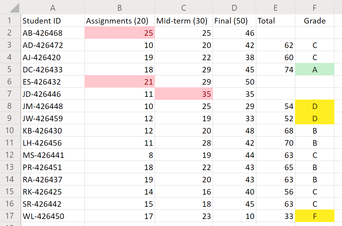
Запустите скрипт калькулятора оценок на единственном листе. Скрипт суммирует оценки и присваивает каждому учащемуся буквенный оценок. Если в каких-либо отдельных оценках больше баллов, чем стоит задание или тест, то оценка, наступающая с ошибкой, помечается красным цветом, а итоговая оценка не вычисляется. Кроме того, все оценки "A" выделены зеленым цветом, а "D" и "F" — желтым.

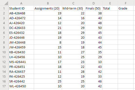
Перед запуском сценария

После выполнения скрипта