適用於: 適用於 Python 的 Azure Machine Learning SDK v1
這很重要
本文提供使用 Azure Machine Learning SDK v1 的相關信息。 SDK v1 自 2025 年 3 月 31 日起已被取代。 其支援將於 2026 年 6 月 30 日結束。 您可以在該日期之前安裝並使用 SDK v1。 您使用 SDK v1 的現有工作流程將在支援終止日期後繼續運作。 不過,如果產品發生架構變更,它們可能會面臨安全性風險或重大變更。
建議您在 2026 年 6 月 30 日之前轉換至 SDK v2。 如需 SDK v2 的詳細資訊,請參閱 什麼是 Azure Machine Learning CLI 和 Python SDK v2? 和 SDK v2 參考。
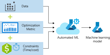
在本文中,您將學習如何使用 Azure Machine Learning 自動化 ML,運用 Azure Machine Learning Python SDK 來定型迴歸模型。 迴歸模型可預測紐約市 (NYC) 營運計程車的乘客車資。 您可以使用 Python SDK 撰寫程式碼並使用備妥的資料來設定工作區、使用自訂數在本機定型模型,以及探索結果。
此程序接受定型資料和組態設定。 它會自動逐一查看不同功能正規化/標準化方法、模型及超參數設定的組合,以獲得最佳模型。 下圖說明迴歸模型定型的處理流程:
必要條件
Azure 訂用帳戶。 您可以建立 Azure Machine Learning 的免費或付費帳戶。
Azure Machine Learning 工作區或計算執行個體。 若要準備這些資源,請參閱快速入門:開始使用 Azure Machine Learning。
將筆記本載入您的工作區,以取得為教學課程練習準備的範例資料:
在 Azure Machine Learning 工作室中前往您的工作區,選取 [筆記本],然後選取 [範例] 索引標籤。
在筆記本清單中,展開 [範例]>[SDK v1]>[教學課程]>[regression-automl-nyc-taxi-data] 節點。
選取 [regression-automated-ml.ipynb] 筆記本。
若要在此教學課程中執行每個筆記本儲存格,請選取 [複製此檔案]。
替代方法:如果您喜歡,可以在本機環境中執行教學課程練習。 本教學課程可在 GitHub 的 Azure Machine Learning 筆記本存放庫中取得。 若使用此方法,請遵循下列步驟以取得必要套件:
在本機電腦上執行
pip install azureml-opendatasets azureml-widgets命令,以取得必要套件。
下載並準備資料
開放資料集套件中有一個類別代表每個資料來源 (例如 NycTlcGreen),可以在下載之前輕鬆篩選日期參數。
下列程式碼會匯入必要套件:
from azureml.opendatasets import NycTlcGreen
import pandas as pd
from datetime import datetime
from dateutil.relativedelta import relativedelta
第一個步驟是建立計程車資料的資料框架。 當您在非 Spark 環境中運作時,開放資料集套件僅允許一次下載一個月的特定類別資料。 此方法有助於避免使用大型資料集時發生 MemoryError 問題。
若要下載計程車資料,請反覆一次擷取一個月的資料。 將下一組資料附加至 green_taxi_df 數據框架之前,請從每個月的資料隨機取樣 2,000 筆記錄,然後預覽資料。 這種方法有助於避免資料框架膨脹。
下列程式碼會建立資料框架、擷取資料並載入資料框架:
green_taxi_df = pd.DataFrame([])
start = datetime.strptime("1/1/2015","%m/%d/%Y")
end = datetime.strptime("1/31/2015","%m/%d/%Y")

for sample_month in range(12):
   temp_df_green = NycTlcGreen(start + relativedelta(months=sample_month), end + relativedelta(months=sample_month)) \
      .to_pandas_dataframe()
   green_taxi_df = green_taxi_df.append(temp_df_green.sample(2000))

green_taxi_df.head(10)
下表顯示範例計程車資料中許多資料列的值:
| vendorID(供應商識別碼) | lpepPickupDatetime | lpepDropoffDatetime | 乘客數量 | 行程距離 | puLocationId | doLocationId | pickupLongitude | 取貨緯度 | dropoffLongitude | ... | 付款類型 | 票價金額 | extra | mtaTax | improvementSurcharge | tipAmount | 通行費金額 | ehailFee | 總金額 | 旅行類型 |
|---|---|---|---|---|---|---|---|---|---|---|---|---|---|---|---|---|---|---|---|---|
| 2 | 2015-01-30 18:38:09 | 2015-01-30 19:01:49 | 1 | 1.88 | 無 | 無 | -73.996155 | 40.690903 | -73.964287 | ... | 1 | 15.0 | 1.0 | 0.5 | 0.3 | 4.00 | 0.0 | 無 | 20.80 | 1.0 |
| 1 | 2015-01-17 23:21:39 | 2015-01-17 23:35:16 | 1 | 2.70 | 無 | 無 | -73.978508 | 40.687984 | -73.955116 | ... | 1 | 11.5 | 0.5 | 0.5 | 0.3 | 2.55 | 0.0 | 無 | 15.35 | 1.0 |
| 2 | 2015-01-16 01:38:40 | 2015-01-16 01:52:55 | 1 | 3.54 | 無 | 無 | -73.957787 | 40.721779 | -73.963005 | ... | 1 | 13.5 | 0.5 | 0.5 | 0.3 | 2.80 | 0.0 | 無 | 17.60 | 1.0 |
| 2 | 2015-01-04 17:09:26 | 2015-01-04 17:16:12 | 1 | 1.00 | 無 | 無 | -73.919914 | 40.826023 | -73.904839 | ... | 2 | 6.5 | 0.0 | 0.5 | 0.3 | 0.00 | 0.0 | 無 | 7.30 | 1.0 |
| 1 | 2015-01-14 10:10:57 | 2015-01-14 10:33:30 | 1 | 5.10 | 無 | 無 | -73.943710 | 40.825439 | -73.982964 | ... | 1 | 18.5 | 0.0 | 0.5 | 0.3 | 3.85 | 0.0 | 無 | 23.15 | 1.0 |
| 2 | 2015-01-19 18:10:41 | 2015-01-19 18:32:20 | 1 | 7.41 | 無 | 無 | -73.940918 | 40.839714 | -73.994339 | ... | 1 | 24.0 | 0.0 | 0.5 | 0.3 | 4.80 | 0.0 | 無 | 29.60 | 1.0 |
| 2 | 2015-01-01 15:44:21 | 2015-01-01 15:50:16 | 1 | 1.03 | 無 | 無 | -73.985718 | 40.685646 | -73.996773 | ... | 1 | 6.5 | 0.0 | 0.5 | 0.3 | 1.30 | 0.0 | 無 | 8.60 | 1.0 |
| 2 | 2015-01-12 08:01:21 | 2015-01-12 08:14:52 | 5 | 2.94 | 無 | 無 | -73.939865 | 40.789822 | -73.952957 | ... | 2 | 12.5 | 0.0 | 0.5 | 0.3 | 0.00 | 0.0 | 無 | 13:30 | 1.0 |
| 1 | 2015-01-16 21:54:26 | 2015-01-16 22:12:39 | 1 | 3.00 | 無 | 無 | -73.957939 | 40.721928 | -73.926247 | ... | 1 | 14.0 | 0.5 | 0.5 | 0.3 | 2.00 | 0.0 | 無 | 下午5點30分 | 1.0 |
| 2 | 2015-01-06 06:34:53 | 2015-01-06 06:44:23 | 1 | 2.31 | 無 | 無 | -73.943825 | 40.810257 | -73.943062 | ... | 1 | 10.0 | 0.0 | 0.5 | 0.3 | 2.00 | 0.0 | 無 | 12.80 | 1.0 |
移除一些您在定型或建置其他功能時不需用到的資料行,會很有幫助。 例如,您可以移除 lpepPickupDatetime 資料行,因為自動化 ML 會自動處理時間型功能。
下列程式碼會從範例資料中移除 14 個資料列:
columns_to_remove = ["lpepDropoffDatetime", "puLocationId", "doLocationId", "extra", "mtaTax",
                "improvementSurcharge", "tollsAmount", "ehailFee", "tripType", "rateCodeID",
                "storeAndFwdFlag", "paymentType", "fareAmount", "tipAmount"
               ]
for col in columns_to_remove:
   green_taxi_df.pop(col)

green_taxi_df.head(5)
清理資料
下一個步驟是清理資料。
下列程式碼會在新的資料框架上執行 describe() 函式,為每個欄位產生摘要統計資料:
green_taxi_df.describe()
下表顯示範例資料中其餘欄位的摘要統計資料:
| vendorID(供應商識別碼) | 乘客數量 | 行程距離 | pickupLongitude | 取貨緯度 | dropoffLongitude | dropoffLatitude | 總金額 | |
|---|---|---|---|---|---|---|---|---|
| 計數 | 24000.00 | 24000.00 | 24000.00 | 24000.00 | 24000.00 | 24000.00 | 24000.00 | 24000.00 |
| 平均值 | 1.777625 | 1.373625 | 2.893981 | -73.827403 | 40.689730 | -73.819670 | 40.684436 | 14.892744 |
| 標準 | 0.415850 | 1.046180 | 3.072343 | 2.821767 | 1.556082 | 2.901199 | 1.599776 | 12.339749 |
| 最小值 | 1.00 | 0.00 | 0.00 | -74.357101 | 0.00 | -74.342766 | 0.00 | -120.80 |
| 25% | 2.00 | 1.00 | 1.05 | -73.959175 | 40.699127 | -73.966476 | 40.699459 | 8.00 |
| 50% | 2.00 | 1.00 | 1.93 | -73.945049 | 40.746754 | -73.944221 | 40.747536 | 11.30 |
| 75% | 2.00 | 1.00 | 3.70 | -73.917089 | 40.803060 | -73.909061 | 40.791526 | 17.80 |
| 最大 | 2.00 | 8.00 | 154.28 | 0.00 | 41.109089 | 0.00 | 40.982826 | 425.00 |
摘要統計資料會顯示幾個極端值欄位,這些值會降低模型的精確度。 若要解決此問題,請篩選緯度/經度 (緯/經) 欄位,以顯示位於曼哈頓區域範圍內的值。 此方法會篩選掉較長途的計程車車程,或與其他特性的關聯性方面屬於極端值的車程。
接下來,請篩選 tripDistance 欄位,找出值大於零、但小於 31 英哩 (兩個經/緯度組之間的半正矢距離) 的資料。 此技術可消除車程成本不一致的長途極端值車程。
最後,篩選掉計程車車資為負值的 totalAmount 欄位,因為這在模型內容中沒有意義。 欄位 passengerCount 也含有不正確的資料,其中最小值為零。
下列程式碼會使用查詢函式,篩選掉這些值異常狀況。 然後,程式碼會移除定型不需要的最後幾個資料行:
final_df = green_taxi_df.query("pickupLatitude>=40.53 and pickupLatitude<=40.88")
final_df = final_df.query("pickupLongitude>=-74.09 and pickupLongitude<=-73.72")
final_df = final_df.query("tripDistance>=0.25 and tripDistance<31")
final_df = final_df.query("passengerCount>0 and totalAmount>0")

columns_to_remove_for_training = ["pickupLongitude", "pickupLatitude", "dropoffLongitude", "dropoffLatitude"]
for col in columns_to_remove_for_training:
   final_df.pop(col)
此順序中的最後一個步驟是再次對資料呼叫 describe() 函式,以確保資料清理如預期般運作。 您現在已準備好一組經過清理的計程車、假日及氣象資料,可供機器學習模型定型使用:
final_df.describe()
設定工作區
從現有的工作區建立工作區物件。 Workspace \(英文\) 是會接受您 Azure 訂用帳戶和資源資訊的類別。 它也會建立雲端資源來監視及追蹤您的模型執行。
下列程式碼會呼叫 Workspace.from_config() 函式來讀取 config.json 檔案,並將驗證詳細資料載入名為 ws 的物件。
from azureml.core.workspace import Workspace
ws = Workspace.from_config()
本教學課程的其餘程式碼均會使用 ws 物件。
將資料分成訓練集和測試集
您可以使用 train_test_split 程式庫中的 函式,將資料分割成訓練集和測試集。 此函式會將資料分成用於模型定型的 x (特性) 資料集,以及用於測試的 y (要預測的值) 資料集。
test_size 參數會決定要配置給測試的資料百分比。
random_state 參數會設定隨機產生器的種子,讓您的「定型-測試」分割具有確定性。
下列程式碼會呼叫 train_test_split 函式,以載入 x 和 y 資料集:
from sklearn.model_selection import train_test_split

x_train, x_test = train_test_split(final_df, test_size=0.2, random_state=223)
此步驟的目的是準備資料點,以測試已完成、但未用來定型模型的模型。 這些點可用來測量真正的精確度。 定型良好的模型是可以從看不見的資料進行精確預測的模型。 您現在已備妥資料,可自動定型機器學習模型。
自動定型模型
若要自動將模型定型,請執行下列步驟:
定義用於實驗執行的設定。 將訓練資料連結至設定,並修改用來控制訓練程序的設定。
提交實驗來調整模型。 提交實驗之後,程序會根據您定義的條件約束,反覆運算不同的機器學習演算法和超參數設定。 它會將精確度計量最佳化,以選擇最適化模型。
定義定型設定
定義用於定型的實驗參數與模型設定。 檢視設定的完整清單。 使用這些預設設定提交實驗大約需要 5-20 分鐘的時間。 若要減少執行階段,請減少 experiment_timeout_hours 參數。
| 屬性 | 本教學課程中的值 | 描述 |
|---|---|---|
iteration_timeout_minutes |
10 | 每次反覆運算的時間限制 (分鐘)。 對於每次反覆運算都需要較多時間的較大資料集,請提高此值。 |
experiment_timeout_hours |
0.3 | 在實驗終止之前,所有反覆運算合在一起所花費的時間量上限 (以小時為單位)。 |
enable_early_stopping |
對 | 此旗標可在分數未在短期內改善時啟用提早終止。 |
primary_metric |
史皮爾曼相關係數 | 您想要最佳化的度量。 最適化模型會根據此計量來選擇。 |
featurization |
自動 | auto 值可讓實驗預先處理輸入資料,包括處理遺漏的資料、將文字轉換成數值等等。 |
verbosity |
logging.INFO | 控制記錄層級。 |
n_cross_validations |
5 | 未指定驗證資料時所要執行的交叉驗證分割數目。 |
下列程式碼會提交實驗:
import logging

automl_settings = {
   "iteration_timeout_minutes": 10,
   "experiment_timeout_hours": 0.3,
   "enable_early_stopping": True,
   "primary_metric": 'spearman_correlation',
   "featurization": 'auto',
   "verbosity": logging.INFO,
   "n_cross_validations": 5
}
下列程式碼可讓您使用您定義的定型設定作為 **kwargs 物件的 AutoMLConfig 參數。 此外,請指定您的訓練資料和模型類型 (在此案例中為 regression)。
from azureml.train.automl import AutoMLConfig

automl_config = AutoMLConfig(task='regression',
                      debug_log='automated_ml_errors.log',
                      training_data=x_train,
                      label_column_name="totalAmount",
                      **automl_settings)
附註
自動化 ML 前置處理步驟 (功能正規化、處理遺漏的資料、將文字轉換成數值等等) 會成為基礎模型的一部分。 使用模型進行預測時,定型期間所套用的相同前置處理步驟會自動套用至您的輸入資料。
定型自動迴歸模型
在您的工作區中建立實驗物件。 實驗作為個別作業的容器。 將已定義的 automl_config 物件傳送至實驗,並將輸出設定為 True,以便在作業期間檢視進度。
開始實驗後,顯示的輸出會隨著實驗執行即時更新。 對於每次反覆運算,您都可以檢視模型類型、執行的持續時間,以及定型精確度。
BEST 欄位會根據計量類型來追蹤執行成效最佳的定型分數:
from azureml.core.experiment import Experiment
experiment = Experiment(ws, "Tutorial-NYCTaxi")
local_run = experiment.submit(automl_config, show_output=True)
輸出如下:
Running on local machine
Parent Run ID: AutoML_1766cdf7-56cf-4b28-a340-c4aeee15b12b
Current status: DatasetFeaturization. Beginning to featurize the dataset.
Current status: DatasetEvaluation. Gathering dataset statistics.
Current status: FeaturesGeneration. Generating features for the dataset.
Current status: DatasetFeaturizationCompleted. Completed featurizing the dataset.
Current status: DatasetCrossValidationSplit. Generating individually featurized CV splits.
Current status: ModelSelection. Beginning model selection.

****************************************************************************************************
ITERATION: The iteration being evaluated.
PIPELINE: A summary description of the pipeline being evaluated.
DURATION: Time taken for the current iteration.
METRIC: The result of computing score on the fitted pipeline.
BEST: The best observed score thus far.
****************************************************************************************************

 ITERATION   PIPELINE                              DURATION     METRIC     BEST
       0   StandardScalerWrapper RandomForest          0:00:16      0.8746   0.8746
       1   MinMaxScaler RandomForest                 0:00:15      0.9468   0.9468
       2   StandardScalerWrapper ExtremeRandomTrees      0:00:09      0.9303   0.9468
       3   StandardScalerWrapper LightGBM             0:00:10      0.9424   0.9468
       4   RobustScaler DecisionTree                 0:00:09      0.9449   0.9468
       5   StandardScalerWrapper LassoLars            0:00:09      0.9440   0.9468
       6   StandardScalerWrapper LightGBM             0:00:10      0.9282   0.9468
       7   StandardScalerWrapper RandomForest          0:00:12      0.8946   0.9468
       8   StandardScalerWrapper LassoLars            0:00:16      0.9439   0.9468
       9   MinMaxScaler ExtremeRandomTrees            0:00:35      0.9199   0.9468
      10   RobustScaler ExtremeRandomTrees            0:00:19      0.9411   0.9468
      11   StandardScalerWrapper ExtremeRandomTrees      0:00:13      0.9077   0.9468
      12   StandardScalerWrapper LassoLars            0:00:15      0.9433   0.9468
      13   MinMaxScaler ExtremeRandomTrees            0:00:14      0.9186   0.9468
      14   RobustScaler RandomForest                 0:00:10      0.8810   0.9468
      15   StandardScalerWrapper LassoLars            0:00:55      0.9433   0.9468
      16   StandardScalerWrapper ExtremeRandomTrees      0:00:13      0.9026   0.9468
      17   StandardScalerWrapper RandomForest          0:00:13      0.9140   0.9468
      18   VotingEnsemble                         0:00:23      0.9471   0.9471
      19   StackEnsemble                          0:00:27      0.9463   0.9471
瀏覽結果
使用 Jupyter 小工具,探索自動定型的結果。 這項小工具允許查看所有個別作業反覆項目的圖表和資料表,並且將正確性計量和中繼資料加以定型。 此外,您也可以使用下拉式清單選取器,來篩選主要計量以外的不同精確度計量。
下列程式碼會產生圖表來探索結果:
from azureml.widgets import RunDetails
RunDetails(local_run).show()
Jupyter Widget 的執行詳細資料:

Jupyter Widget 的圖表:

擷取最佳模型
下列程式碼可讓您從反覆運算中選取最佳模型。
get_output 函式會傳回最佳執行和上一個配適引動過程的配適模型。 藉由在 get_output 函式上使用多載,您可以針對任何已記錄的計量或特定的反覆運算,擷取執行成效最佳的適合模型。
best_run, fitted_model = local_run.get_output()
print(best_run)
print(fitted_model)
測試最佳模型精確度
使用最佳模型在測試資料集上執行預測,以預測計程車車資。 函式 predict 使用最佳模型,並依據 資料集預測 y 值 (x_test)。
下列程式碼會列印 y_predict 資料集中的前 10 個預測成本值:
y_test = x_test.pop("totalAmount")

y_predict = fitted_model.predict(x_test)
print(y_predict[:10])
計算結果的 root mean squared error。 將 y_test 資料框架轉換為清單,與預測值進行比較。
mean_squared_error 函式採用兩個值陣列,並計算這兩個陣列之間的平均平方誤差。 取結果的平方根會產生與 y 變數 (成本) 相同單位的誤差。 這大致上可表示計程車車資預測與實際車資的差距。
from sklearn.metrics import mean_squared_error
from math import sqrt

y_actual = y_test.values.flatten().tolist()
rmse = sqrt(mean_squared_error(y_actual, y_predict))
rmse
執行下列程式碼,以使用完整的 y_actual 和 y_predict 資料集來計算平均絕對百分比誤差 (MAPE)。 此計量會計算每個預測值與實際值之間的絕對差異,並加總所有差異。 然後它會以實際值總計的百分比來表示該總和。
sum_actuals = sum_errors = 0

for actual_val, predict_val in zip(y_actual, y_predict):
   abs_error = actual_val - predict_val
   if abs_error < 0:
      abs_error = abs_error * -1

   sum_errors = sum_errors + abs_error
   sum_actuals = sum_actuals + actual_val

mean_abs_percent_error = sum_errors / sum_actuals
print("Model MAPE:")
print(mean_abs_percent_error)
print()
print("Model Accuracy:")
print(1 - mean_abs_percent_error)
輸出如下:
Model MAPE:
0.14353867606052823

Model Accuracy:
0.8564613239394718
從這兩個預測精確度計量中,您會看到模型從資料集的特性預測計程車車資的表現相當不錯,大多在 +- 4.00 美元以內,誤差約為 15%。
傳統的機器學習模型開發程序需要大量資源。 它需要大量的領域知識和時間投資,才能執行和比較數十個模型的結果。 使用自動化機器學習,是您針對個人案例快速測試許多不同模型的絕佳方式。
清理資源
如果您不打算使用其他 Azure Machine Learning 教學課程,請完成下列步驟以移除不再需要的資源。
停止計算
如果您使用計算,您可以在不使用虛擬機器時停止機器,以降低成本:
移至 Azure Machine Learning 工作室中的工作區,然後選取 [計算]。
在清單中,選取您要停止的計算,然後選取 [停止]。
當您準備好再次使用計算時,可以重新啟動虛擬機器。
刪除其他資源
如果您不打算使用在本教學課程中建立的資源,可以刪除它們,避免產生進一步的費用。
請遵循下列步驟來移除資源群組和所有資源:
在 Azure 入口網站中,移至資源群組。
在清單中,選取您在本教學課程中建立的資源群組,然後選取 [刪除資源群組]。
在確認提示中,輸入資源群組名稱,然後選取 [刪除]。
如果您想保留該資源群組,且只刪除單一工作區,請遵循下列步驟:
在 Azure 入口網站中,移至您要移除的工作區所在的資源群組。
選取該工作區,選取 [屬性],然後選取 [刪除]。