使用 Apache Spark 和 Python 分析數據
在本教學課程中,您將瞭解如何使用 Azure 開放數據集和 Apache Spark 來執行探勘數據分析。
特別是,我們將分析 紐約市 (NYC) 計程車 數據集。 數據可透過 Azure 開放資料集取得。 此數據集子集包含黃色計程車車程的相關信息:每個車程的相關信息、開始和結束時間和位置、成本和其他有趣的屬性。
必要條件
取得 Microsoft Fabric 訂用 帳戶。 或者,註冊免費的 Microsoft Fabric 試用版。
登入 Microsoft Fabric。
使用首頁左側的體驗切換器,切換至 Synapse 資料科學 體驗。
下載並準備數據
使用 PySpark 建立筆記本。 如需指示,請參閱 建立筆記本。
注意
由於 PySpark 核心,您不需要明確地建立任何內容。 當您執行第一個程式代碼數據格時,系統會自動為您建立Spark內容。
在本教學課程中,我們將使用數個不同的連結庫來協助我們可視化數據集。 若要執行這項分析,請匯入下列連結庫:
import matplotlib.pyplot as plt
import seaborn as sns
import pandas as pd
由於原始數據採用 Parquet 格式,因此您可以使用 Spark 內容,將檔案直接提取到記憶體中做為 DataFrame。 透過開放式數據集 API 擷取數據來建立 Spark 數據框架。 在這裡,我們會在讀取屬性上使用Spark DataFrame架構來推斷數據類型和架構。
from azureml.opendatasets import NycTlcYellow

end_date = parser.parse('2018-06-06')
start_date = parser.parse('2018-05-01')
nyc_tlc = NycTlcYellow(start_date=start_date, end_date=end_date)
nyc_tlc_pd = nyc_tlc.to_pandas_dataframe()

df = spark.createDataFrame(nyc_tlc_pd)
讀取數據之後,我們想要執行一些初始篩選來清除數據集。 我們可能會移除不必要的數據行,並新增擷取重要資訊的數據行。 此外,我們會篩選出數據集內的異常狀況。
# Filter the dataset
from pyspark.sql.functions import *

filtered_df = df.select('vendorID', 'passengerCount', 'tripDistance','paymentType', 'fareAmount', 'tipAmount'\
                                , date_format('tpepPickupDateTime', 'hh').alias('hour_of_day')\
                                , dayofweek('tpepPickupDateTime').alias('day_of_week')\
                                , dayofmonth(col('tpepPickupDateTime')).alias('day_of_month'))\
                            .filter((df.passengerCount > 0)\
                                & (df.tipAmount >= 0)\
                                & (df.fareAmount >= 1) & (df.fareAmount <= 250)\
                                & (df.tripDistance > 0) & (df.tripDistance <= 200))

filtered_df.createOrReplaceTempView("taxi_dataset")
分析資料
身為數據分析師,您有各種不同的工具可協助您從數據中擷取見解。 在本教學課程的這個部分中,我們將逐步解說一些 Microsoft Fabric 筆記本中可用的實用工具。 在此分析中,我們想要瞭解在所選期間產生較高計程車小費的因素。
Apache Spark SQL Magic
首先,我們將使用 Microsoft Fabric 筆記本,執行 Apache Spark SQL 和 magic 命令的探勘數據分析。 取得查詢之後,我們將使用內 chart options 建功能將結果可視化。
在您的筆記本中,建立新的數據格,並複製下列程序代碼。 藉由使用此查詢,我們想要瞭解平均小費金額在選取期間變更的方式。 此查詢也會協助我們識別其他有用的見解,包括每日最低/最大小費金額和平均票價金額。
%%sql
SELECT
    day_of_month
    , MIN(tipAmount) AS minTipAmount
    , MAX(tipAmount) AS maxTipAmount
    , AVG(tipAmount) AS avgTipAmount
    , AVG(fareAmount) as fareAmount
FROM taxi_dataset
GROUP BY day_of_month
ORDER BY day_of_month ASC
查詢完成執行之後,我們可以切換至圖表檢視來可視化結果。 這個範例會藉由將字段指定
day_of_month為索引鍵和avgTipAmount值,以建立折線圖。 選取選取項目之後,請選取 [ 套用 ] 以重新整理您的圖表。
顯現資料
除了內建的筆記本圖表選項之外,您還可以使用熱門的開放原始碼連結庫來建立自己的視覺效果。 在下列範例中,我們將使用 Seaborn 和 Matplotlib。 這些通常是用於數據視覺效果的 Python 連結庫。
為了讓開發變得更容易且成本較低,我們會向下取樣數據集。 我們將使用內建的 Apache Spark 取樣功能。 此外,Seaborn 和 Matplotlib 都需要 Pandas DataFrame 或 NumPy 陣列。 若要取得 Pandas DataFrame,請使用
toPandas()命令來轉換 DataFrame。# To make development easier, faster, and less expensive, downsample for now sampled_taxi_df = filtered_df.sample(True, 0.001, seed=1234) # The charting package needs a Pandas DataFrame or NumPy array to do the conversion sampled_taxi_pd_df = sampled_taxi_df.toPandas()我們想要了解數據集中的秘訣分佈。 我們將使用 Matplotlib 來建立直方圖,以顯示小費數量和計數的分佈。 根據分佈,我們可以看到提示會偏向小於或等於 $10 的金額。
# Look at a histogram of tips by count by using Matplotlib

ax1 = sampled_taxi_pd_df['tipAmount'].plot(kind='hist', bins=25, facecolor='lightblue')
ax1.set_title('Tip amount distribution')
ax1.set_xlabel('Tip Amount ($)')
ax1.set_ylabel('Counts')
plt.suptitle('')
plt.show()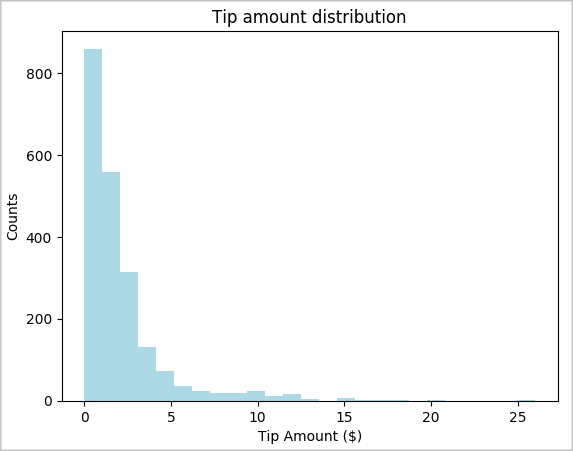
接下來,我們想要瞭解指定車程的秘訣與星期幾之間的關聯性。 使用 Seaborn 來建立方塊圖,以摘要說明每周每一天的趨勢。
# View the distribution of tips by day of week using Seaborn
ax = sns.boxplot(x="day_of_week", y="tipAmount",data=sampled_taxi_pd_df, showfliers = False)
ax.set_title('Tip amount distribution per day')
ax.set_xlabel('Day of Week')
ax.set_ylabel('Tip Amount ($)')
plt.show()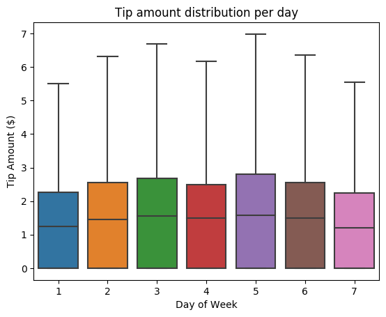
我們的另一個假設可能是乘客數目與計程車小費總額之間有積極關係。 若要確認此關聯性,請執行下列程式代碼來產生方塊圖,以說明每個乘客計數的秘訣分佈。
# How many passengers tipped by various amounts
ax2 = sampled_taxi_pd_df.boxplot(column=['tipAmount'], by=['passengerCount'])
ax2.set_title('Tip amount by Passenger count')
ax2.set_xlabel('Passenger count')
ax2.set_ylabel('Tip Amount ($)')
ax2.set_ylim(0,30)
plt.suptitle('')
plt.show()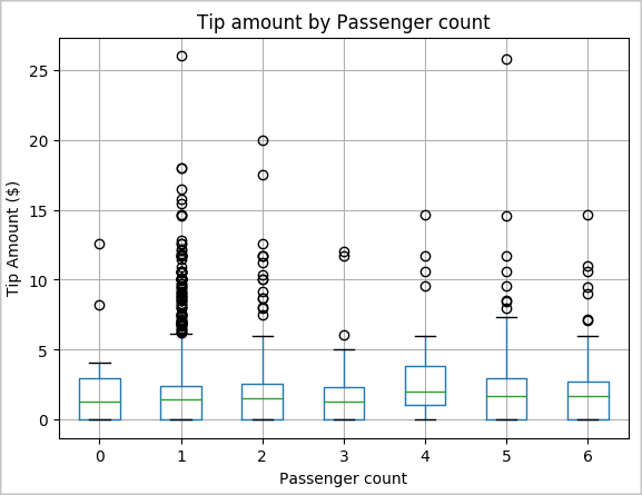
最後,我們想要瞭解票價金額與小費金額之間的關聯性。 根據結果,我們可以看到有數個觀察,人們沒有提示。 不過,我們也看到整體票價與小費金額之間的積極關係。
# Look at the relationship between fare and tip amounts

ax = sampled_taxi_pd_df.plot(kind='scatter', x= 'fareAmount', y = 'tipAmount', c='blue', alpha = 0.10, s=2.5*(sampled_taxi_pd_df['passengerCount']))
ax.set_title('Tip amount by Fare amount')
ax.set_xlabel('Fare Amount ($)')
ax.set_ylabel('Tip Amount ($)')
plt.axis([-2, 80, -2, 20])
plt.suptitle('')
plt.show()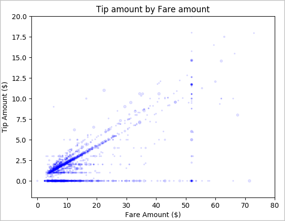
相關內容
- 瞭解如何在 Apache Spark 上使用 Pandas API: Apache Spark 上的 Pandas API
- Python 內嵌安裝
意見反應
即將登場:在 2024 年,我們將逐步淘汰 GitHub 問題作為內容的意見反應機制,並將它取代為新的意見反應系統。 如需詳細資訊,請參閱:https://aka.ms/ContentUserFeedback。
提交並檢視相關的意見反應