Tutorial: create, evaluate, and score a machine fault detection model
This tutorial presents an end-to-end example of a Synapse Data Science workflow in Microsoft Fabric. The scenario uses machine learning for a more systematic approach to fault diagnosis, to proactively identify issues and to take actions before an actual machine failure. The goal is to predict whether a machine would experience a failure based on process temperature, rotational speed, etc.
This tutorial covers these steps:
- Install custom libraries
- Load and process the data
- Understand the data through exploratory data analysis
- Use scikit-learn, LightGBM, and MLflow to train machine learning models, and use the Fabric Autologging feature to track experiments
- Score the trained models with the Fabric
PREDICTfeature, save the best model, and load that model for predictions - Show the loaded model performance with Power BI visualizations
Prerequisites
Get a Microsoft Fabric subscription. Or, sign up for a free Microsoft Fabric trial.
Sign in to Microsoft Fabric.
Use the experience switcher on the left side of your home page to switch to the Synapse Data Science experience.
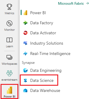
- If necessary, create a Microsoft Fabric lakehouse as described in Create a lakehouse in Microsoft Fabric.
Follow along in a notebook
You can choose one of these options to follow along in a notebook:
- Open and run the built-in notebook in the Data Science experience
- Upload your notebook from GitHub to the Data Science experience
Open the built-in notebook
The sample Machine failure notebook accompanies this tutorial.
To open the tutorial's built-in sample notebook in the Synapse Data Science experience:
Go to the Synapse Data Science home page.
Select Use a sample.
Select the corresponding sample:
- From the default End-to-end workflows (Python) tab, if the sample is for a Python tutorial.
- From the End-to-end workflows (R) tab, if the sample is for an R tutorial.
- From the Quick tutorials tab, if the sample is for a quick tutorial.
Attach a lakehouse to the notebook before you start running code.
Import the notebook from GitHub
The AISample - Predictive Maintenance notebook accompanies this tutorial.
To open the accompanying notebook for this tutorial, follow the instructions in Prepare your system for data science tutorials, to import the notebook to your workspace.
If you'd rather copy and paste the code from this page, you can create a new notebook.
Be sure to attach a lakehouse to the notebook before you start running code.
Step 1: Install custom libraries
For machine learning model development or ad-hoc data analysis, you might need to quickly install a custom library for your Apache Spark session. You have two options to install libraries.
- Use the inline installation capabilities (
%pipor%conda) of your notebook to install a library, in your current notebook only. - Alternatively, you can create a Fabric environment, install libraries from public sources or upload custom libraries to it, and then your workspace admin can attach the environment as the default for the workspace. All the libraries in the environment will then become available for use in any notebooks and Spark job definitions in the workspace. For more information on environments, see create, configure, and use an environment in Microsoft Fabric.
For this tutorial, use %pip install to install the imblearn library in your notebook.
Note
The PySpark kernel restarts after %pip install runs. Install the needed libraries before you run any other cells.
# Use pip to install imblearn
%pip install imblearn
Step 2: Load the data
The dataset simulates logging of a manufacturing machine's parameters as a function of time, which is common in industrial settings. It consists of 10,000 data points stored as rows with features as columns. The features include:
A Unique Identifier (UID) that ranges from 1 to 10000
Product ID, consisting of a letter L (for low), M (for medium), or H (for high), to indicate the product quality variant, and a variant-specific serial number. Low, medium, and high-quality variants make up 60%, 30%, and 10% of all products, respectively
Air temperature, in degrees Kelvin (K)
Process Temperature, in degrees Kelvin
Rotational Speed, in revolutions per minute (RPM)
Torque, in Newton-Meters (Nm)
Tool wear, in minutes. The quality variants H, M, and L add 5, 3, and 2 minutes of tool wear respectively to the tool used in the process
A Machine Failure Label, to indicate whether the machine failed in the specific data point. This specific data point can have any of the following five independent failure modes:
- Tool Wear Failure (TWF): the tool is replaced or fails at a randomly selected tool wear time, between 200 and 240 minutes
- Heat Dissipation Failure (HDF): heat dissipation causes a process failure if the difference between the air temperature and the process temperature is less than 8.6 K, and the tool's rotational speed is less than 1380 RPM
- Power Failure (PWF): the product of torque and rotational speed (in rad/s) equals the power required for the process. The process fails if this power falls below 3,500 W or exceeds 9,000 W
- OverStrain Failure (OSF): if the product of tool wear and torque exceeds 11,000 minimum Nm for the L product variant (12,000 for M, 13,000 for H), the process fails due to overstrain
- Random Failures (RNF): each process has a failure chance of 0.1%, regardless of the process parameters
Note
If at least one of the above failure modes is true, the process fails, and the "machine failure" label is set to 1. The machine learning method can't determine which failure mode caused the process failure.
Download the dataset and upload to the lakehouse
Connect to the Azure Open Datasets container, and load the Predictive Maintenance dataset. This code downloads a publicly available version of the dataset, and then stores it in a Fabric lakehouse:
Important
Add a lakehouse to the notebook before you run it. Otherwise, you'll get an error. For information about adding a lakehouse, see Connect lakehouses and notebooks.
# Download demo data files into the lakehouse if they don't exist
import os, requests
DATA_FOLDER = "Files/predictive_maintenance/"  # Folder that contains the dataset
DATA_FILE = "predictive_maintenance.csv"  # Data file name
remote_url = "https://synapseaisolutionsa.blob.core.windows.net/public/MachineFaultDetection"
file_list = ["predictive_maintenance.csv"]
download_path = f"/lakehouse/default/{DATA_FOLDER}/raw"

if not os.path.exists("/lakehouse/default"):
    raise FileNotFoundError(
        "Default lakehouse not found, please add a lakehouse and restart the session."
    )
os.makedirs(download_path, exist_ok=True)
for fname in file_list:
    if not os.path.exists(f"{download_path}/{fname}"):
        r = requests.get(f"{remote_url}/{fname}", timeout=30)
        with open(f"{download_path}/{fname}", "wb") as f:
            f.write(r.content)
print("Downloaded demo data files into lakehouse.")
After you download the dataset into the lakehouse, you can load it as a Spark DataFrame:
df = (
    spark.read.option("header", True)
    .option("inferSchema", True)
    .csv(f"{DATA_FOLDER}raw/{DATA_FILE}")
    .cache()
)
df.show(5)
This table shows a preview of the data:
| UDI | Product ID | Type | Air temperature [K] | Process temperature [K] | Rotational speed [rpm] | Torque [Nm] | Tool wear [min] | Target | Failure Type |
|---|---|---|---|---|---|---|---|---|---|
| 1 | M14860 | M | 298.1 | 308.6 | 1551 | 42.8 | 0 | 0 | No Failure |
| 2 | L47181 | L | 298.2 | 308.7 | 1408 | 46.3 | 3 | 0 | No Failure |
| 3 | L47182 | L | 298.1 | 308.5 | 1498 | 49.4 | 5 | 0 | No Failure |
| 4 | L47183 | L | 298.2 | 308.6 | 1433 | 39.5 | 7 | 0 | No Failure |
| 5 | L47184 | L | 298.2 | 308.7 | 1408 | 40.0 | 9 | 0 | No Failure |
Write a Spark DataFrame to a lakehouse delta table
Format the data (for example, replace the spaces with underscores) to facilitate Spark operations in subsequent steps:
# Replace the space in the column name with an underscore to avoid an invalid character while saving
df = df.toDF(*(c.replace(' ', '_') for c in df.columns))
table_name = "predictive_maintenance_data"
df.show(5)
This table shows a preview of the data with reformatted column names:
| UDI | Product_ID | Type | Air_temperature_[K] | Process_temperature_[K] | Rotational_speed_[rpm] | Torque_[Nm] | Tool_wear_[min] | Target | Failure_Type |
|---|---|---|---|---|---|---|---|---|---|
| 1 | M14860 | M | 298.1 | 308.6 | 1551 | 42.8 | 0 | 0 | No Failure |
| 2 | L47181 | L | 298.2 | 308.7 | 1408 | 46.3 | 3 | 0 | No Failure |
| 3 | L47182 | L | 298.1 | 308.5 | 1498 | 49.4 | 5 | 0 | No Failure |
| 4 | L47183 | L | 298.2 | 308.6 | 1433 | 39.5 | 7 | 0 | No Failure |
| 5 | L47184 | L | 298.2 | 308.7 | 1408 | 40.0 | 9 | 0 | No Failure |
# Save data with processed columns to the lakehouse
df.write.mode("overwrite").format("delta").save(f"Tables/{table_name}")
print(f"Spark DataFrame saved to delta table: {table_name}")
Step 3: Preprocess data and perform exploratory data analysis
Convert the Spark DataFrame to a pandas DataFrame, to use Pandas-compatible popular plotting libraries.
Tip
For a large dataset, you might need to load a portion of that dataset.
data = spark.read.format("delta").load("Tables/predictive_maintenance_data")
SEED = 1234
df = data.toPandas()
df.drop(['UDI', 'Product_ID'],axis=1,inplace=True)
# Rename the Target column to IsFail
df = df.rename(columns = {'Target': "IsFail"})
df.info()
Convert specific columns of the dataset to floats or integer types as required, and map strings ('L', 'M', 'H') to numerical values (0, 1, 2):
# Convert temperature, rotational speed, torque, and tool wear columns to float
df['Air_temperature_[K]'] = df['Air_temperature_[K]'].astype(float)
df['Process_temperature_[K]'] = df['Process_temperature_[K]'].astype(float)
df['Rotational_speed_[rpm]'] = df['Rotational_speed_[rpm]'].astype(float)
df['Torque_[Nm]'] = df['Torque_[Nm]'].astype(float)
df['Tool_wear_[min]'] = df['Tool_wear_[min]'].astype(float)

# Convert the 'Target' column to an integer
df['IsFail'] = df['IsFail'].astype(int)
# Map 'L', 'M', 'H' to numerical values
df['Type'] = df['Type'].map({'L': 0, 'M': 1, 'H': 2})
Explore data through visualizations
# Import packages and set plotting style
import seaborn as sns
import matplotlib.pyplot as plt
import pandas as pd
sns.set_style('darkgrid')

# Create the correlation matrix
corr_matrix = df.corr(numeric_only=True)

# Plot a heatmap
plt.figure(figsize=(10, 8))
sns.heatmap(corr_matrix, annot=True)
plt.show()
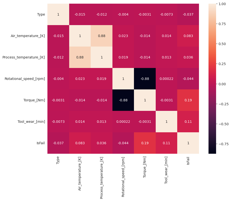
As expected, failure (IsFail) correlates with the selected features (columns). The correlation matrix shows that Air_temperature, Process_temperature, Rotational_speed, Torque, and Tool_wear have the highest correlation with the IsFail variable.
# Plot histograms of select features
fig, axes = plt.subplots(2, 3, figsize=(18,10))
columns = ['Air_temperature_[K]', 'Process_temperature_[K]', 'Rotational_speed_[rpm]', 'Torque_[Nm]', 'Tool_wear_[min]']
data=df.copy()
for ind, item in enumerate (columns):
    column = columns[ind]
    df_column = data[column]
    df_column.hist(ax = axes[ind%2][ind//2], bins=32).set_title(item)
fig.supylabel('count')
fig.subplots_adjust(hspace=0.2)
fig.delaxes(axes[1,2])
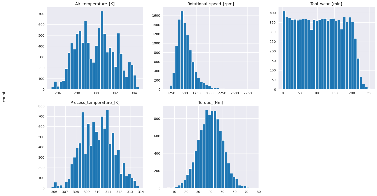
As the plotted graphs show, the Air_temperature, Process_temperature, Rotational_speed, Torque, and Tool_wear variables aren't sparse. They seem to have good continuity in the feature space. These plots confirm that training a machine learning model on this dataset likely produces reliable results that can generalize to a new dataset.
Inspect the target variable for class imbalance
Count the number of samples for failed and unfailed machines, and inspect the data balance for each class (IsFail=0, IsFail=1):
# Plot the counts for no failure and each failure type
plt.figure(figsize=(12, 2))
ax = sns.countplot(x='Failure_Type', data=df)
for p in ax.patches:
    ax.annotate(f'{p.get_height()}', (p.get_x()+0.4, p.get_height()+50))

plt.show()

# Plot the counts for no failure versus the sum of all failure types
plt.figure(figsize=(4, 2))
ax = sns.countplot(x='IsFail', data=df)
for p in ax.patches:
    ax.annotate(f'{p.get_height()}', (p.get_x()+0.4, p.get_height()+50))

plt.show()
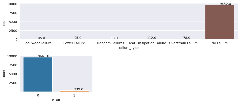
The plots indicate that the no-failure class (shown as IsFail=0 in the second plot) constitutes most of the samples. Use an oversampling technique to create a more balanced training dataset:
# Separate features and target
features = df[['Type', 'Air_temperature_[K]', 'Process_temperature_[K]', 'Rotational_speed_[rpm]', 'Torque_[Nm]', 'Tool_wear_[min]']]
labels = df['IsFail']

# Split the dataset into the training and testing sets
from sklearn.model_selection import train_test_split
X_train, X_test, y_train, y_test = train_test_split(features, labels, test_size=0.2, random_state=42)

# Ignore warnings
import warnings
warnings.filterwarnings('ignore')
# Save test data to the lakehouse for use in future sections
table_name = "predictive_maintenance_test_data"
df_test_X = spark.createDataFrame(X_test)
df_test_X.write.mode("overwrite").format("delta").save(f"Tables/{table_name}")
print(f"Spark DataFrame saved to delta table: {table_name}")
Oversample to balance classes in the training dataset
The previous analysis showed that the dataset is highly imbalanced. That imbalance becomes a problem, because the minority class has too few examples for the model to effectively learn the decision boundary.
SMOTE can solve the problem. SMOTE is a widely used oversampling technique that generates synthetic examples. It generates examples for the minority class based on the Euclidian distances between data points. This method differs from random oversampling, because it creates new examples that don't just duplicate the minority class. The method becomes a more effective technique to handle imbalanced datasets.
# Disable MLflow autologging because you don't want to track SMOTE fitting
import mlflow

mlflow.autolog(disable=True)

from imblearn.combine import SMOTETomek
smt = SMOTETomek(random_state=SEED)
X_train_res, y_train_res = smt.fit_resample(X_train, y_train)

# Plot the counts for both classes
plt.figure(figsize=(4, 2))
ax = sns.countplot(x='IsFail', data=pd.DataFrame({'IsFail': y_train_res.values}))
for p in ax.patches:
    ax.annotate(f'{p.get_height()}', (p.get_x()+0.4, p.get_height()+50))

plt.show()
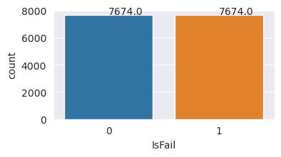
You successfully balanced the dataset. You can now move to model training.
Step 4: Train and evaluate the models
MLflow registers models, trains and compares various models, and picks the best model for prediction purposes. You can use the following three models for model training:
- Random forest classifier
- Logistic regression classifier
- XGBoost classifier
Train a random forest classifier
import numpy as np
from sklearn.ensemble import RandomForestClassifier
from mlflow.models.signature import infer_signature
from sklearn.metrics import f1_score, accuracy_score, recall_score

mlflow.set_experiment("Machine_Failure_Classification")
mlflow.autolog(exclusive=False) # This is needed to override the preconfigured autologging behavior

with mlflow.start_run() as run:
    rfc_id = run.info.run_id
    print(f"run_id {rfc_id}, status: {run.info.status}")
    rfc = RandomForestClassifier(max_depth=5, n_estimators=50)
    rfc.fit(X_train_res, y_train_res)
    signature = infer_signature(X_train_res, y_train_res)

    mlflow.sklearn.log_model(
        rfc,
        "machine_failure_model_rf",
        signature=signature,
        registered_model_name="machine_failure_model_rf"
    )

    y_pred_train = rfc.predict(X_train)
    # Calculate the classification metrics for test data
    f1_train = f1_score(y_train, y_pred_train, average='weighted')
    accuracy_train = accuracy_score(y_train, y_pred_train)
    recall_train = recall_score(y_train, y_pred_train, average='weighted')

    # Log the classification metrics to MLflow
    mlflow.log_metric("f1_score_train", f1_train)
    mlflow.log_metric("accuracy_train", accuracy_train)
    mlflow.log_metric("recall_train", recall_train)

    # Print the run ID and the classification metrics
    print("F1 score_train:", f1_train)
    print("Accuracy_train:", accuracy_train)
    print("Recall_train:", recall_train)

    y_pred_test = rfc.predict(X_test)
    # Calculate the classification metrics for test data
    f1_test = f1_score(y_test, y_pred_test, average='weighted')
    accuracy_test = accuracy_score(y_test, y_pred_test)
    recall_test = recall_score(y_test, y_pred_test, average='weighted')

    # Log the classification metrics to MLflow
    mlflow.log_metric("f1_score_test", f1_test)
    mlflow.log_metric("accuracy_test", accuracy_test)
    mlflow.log_metric("recall_test", recall_test)

    # Print the classification metrics
    print("F1 score_test:", f1_test)
    print("Accuracy_test:", accuracy_test)
    print("Recall_test:", recall_test)
From the output, both the training and test datasets yield an F1 score, accuracy and recall of about 0.9 when using the random forest classifier.
Train a logistic regression classifier
from sklearn.linear_model import LogisticRegression

with mlflow.start_run() as run:
    lr_id = run.info.run_id
    print(f"run_id {lr_id}, status: {run.info.status}")
    lr = LogisticRegression(random_state=42)
    lr.fit(X_train_res, y_train_res)
    signature = infer_signature(X_train_res, y_train_res)

    mlflow.sklearn.log_model(
        lr,
        "machine_failure_model_lr",
        signature=signature,
        registered_model_name="machine_failure_model_lr"
    )

    y_pred_train = lr.predict(X_train)
    # Calculate the classification metrics for training data
    f1_train = f1_score(y_train, y_pred_train, average='weighted')
    accuracy_train = accuracy_score(y_train, y_pred_train)
    recall_train = recall_score(y_train, y_pred_train, average='weighted')

    # Log the classification metrics to MLflow
    mlflow.log_metric("f1_score_train", f1_train)
    mlflow.log_metric("accuracy_train", accuracy_train)
    mlflow.log_metric("recall_train", recall_train)

    # Print the run ID and the classification metrics
    print("F1 score_train:", f1_train)
    print("Accuracy_train:", accuracy_train)
    print("Recall_train:", recall_train)

    y_pred_test = lr.predict(X_test)
    # Calculate the classification metrics for test data
    f1_test = f1_score(y_test, y_pred_test, average='weighted')
    accuracy_test = accuracy_score(y_test, y_pred_test)
    recall_test = recall_score(y_test, y_pred_test, average='weighted')

    # Log the classification metrics to MLflow
    mlflow.log_metric("f1_score_test", f1_test)
    mlflow.log_metric("accuracy_test", accuracy_test)
    mlflow.log_metric("recall_test", recall_test)
Train an XGBoost classifier
from xgboost import XGBClassifier

with mlflow.start_run() as run:
    xgb = XGBClassifier()
    xgb_id = run.info.run_id
    print(f"run_id {xgb_id}, status: {run.info.status}")
    xgb.fit(X_train_res.to_numpy(), y_train_res.to_numpy())
    signature = infer_signature(X_train_res, y_train_res)

    mlflow.xgboost.log_model(
        xgb,
        "machine_failure_model_xgb",
        signature=signature,
        registered_model_name="machine_failure_model_xgb"
    )

    y_pred_train = xgb.predict(X_train)
    # Calculate the classification metrics for training data
    f1_train = f1_score(y_train, y_pred_train, average='weighted')
    accuracy_train = accuracy_score(y_train, y_pred_train)
    recall_train = recall_score(y_train, y_pred_train, average='weighted')

    # Log the classification metrics to MLflow
    mlflow.log_metric("f1_score_train", f1_train)
    mlflow.log_metric("accuracy_train", accuracy_train)
    mlflow.log_metric("recall_train", recall_train)

    # Print the run ID and the classification metrics
    print("F1 score_train:", f1_train)
    print("Accuracy_train:", accuracy_train)
    print("Recall_train:", recall_train)

    y_pred_test = xgb.predict(X_test)
    # Calculate the classification metrics for test data
    f1_test = f1_score(y_test, y_pred_test, average='weighted')
    accuracy_test = accuracy_score(y_test, y_pred_test)
    recall_test = recall_score(y_test, y_pred_test, average='weighted')

    # Log the classification metrics to MLflow
    mlflow.log_metric("f1_score_test", f1_test)
    mlflow.log_metric("accuracy_test", accuracy_test)
    mlflow.log_metric("recall_test", recall_test)
Step 5: Select the best model and predict outputs
In the previous section, you trained three different classifiers: random forest, logistic regression, and XGBoost. You now have the choice to either programmatically access the results, or use the user interface (UI).
For the UI path option, navigate to your workspace and filter the models.
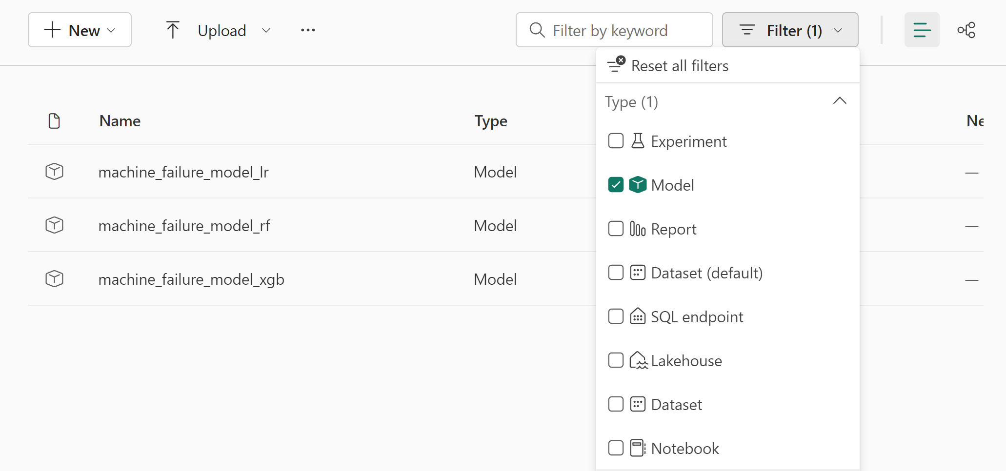
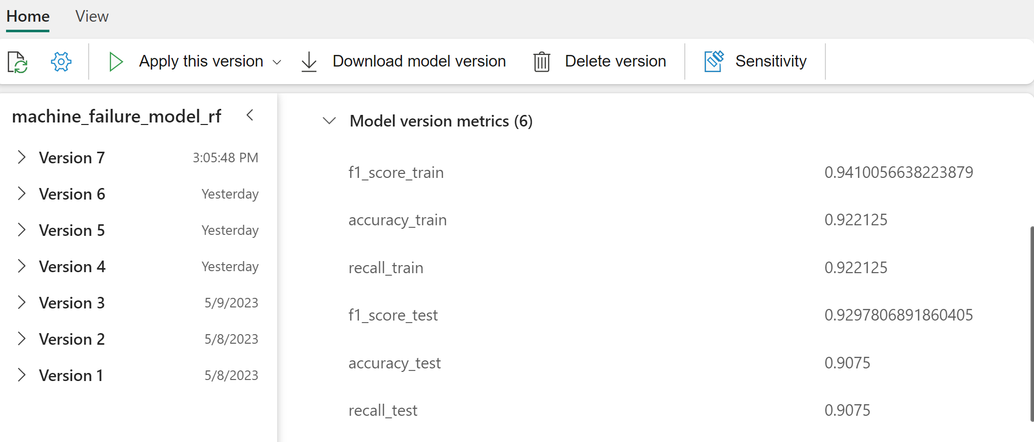
Select individual models for details of the model performance.
This example shows how to programmatically access the models through MLflow:
runs = {'random forest classifier':   rfc_id,
        'logistic regression classifier': lr_id,
        'xgboost classifier': xgb_id}

# Create an empty DataFrame to hold the metrics
df_metrics = pd.DataFrame()

# Loop through the run IDs and retrieve the metrics for each run
for run_name, run_id in runs.items():
    metrics = mlflow.get_run(run_id).data.metrics
    metrics["run_name"] = run_name
    df_metrics = df_metrics.append(metrics, ignore_index=True)

# Print the DataFrame
print(df_metrics)
Although XGBoost yields the best results on the training set, it performs poorly on the test data set. That poor performance indicates over-fitting. The logistic regression classifier performs poorly on both training and test datasets. Overall, random forest strikes a good balance between training performance and avoidance of overfitting.
In the next section, choose the registered random forest model, and perform a prediction with the PREDICT feature:
from synapse.ml.predict import MLFlowTransformer

model = MLFlowTransformer(
    inputCols=list(X_test.columns),
    outputCol='predictions',
    modelName='machine_failure_model_rf',
    modelVersion=1
)
With the MLFlowTransformer object you created to load the model for inferencing, use the Transformer API to score the model on the test dataset:
predictions = model.transform(spark.createDataFrame(X_test))
predictions.show()
This table shows the output:
| Type | Air_temperature_[K] | Process_temperature_[K] | Rotational_speed_[rpm] | Torque_[Nm] | Tool_wear_[min] | predictions |
|---|---|---|---|---|---|---|
| 0 | 300.6 | 309.7 | 1639.0 | 30.4 | 121.0 | 0 |
| 0 | 303.9 | 313.0 | 1551.0 | 36.8 | 140.0 | 0 |
| 1 | 299.1 | 308.6 | 1491.0 | 38.5 | 166.0 | 0 |
| 0 | 300.9 | 312.1 | 1359.0 | 51.7 | 146.0 | 1 |
| 0 | 303.7 | 312.6 | 1621.0 | 38.8 | 182.0 | 0 |
| 0 | 299.0 | 310.3 | 1868.0 | 24.0 | 221.0 | 1 |
| 2 | 297.8 | 307.5 | 1631.0 | 31.3 | 124.0 | 0 |
| 0 | 297.5 | 308.2 | 1327.0 | 56.5 | 189.0 | 1 |
| 0 | 301.3 | 310.3 | 1460.0 | 41.5 | 197.0 | 0 |
| 2 | 297.6 | 309.0 | 1413.0 | 40.2 | 51.0 | 0 |
| 1 | 300.9 | 309.4 | 1724.0 | 25.6 | 119.0 | 0 |
| 0 | 303.3 | 311.3 | 1389.0 | 53.9 | 39.0 | 0 |
| 0 | 298.4 | 307.9 | 1981.0 | 23.2 | 16.0 | 0 |
| 0 | 299.3 | 308.8 | 1636.0 | 29.9 | 201.0 | 0 |
| 1 | 298.1 | 309.2 | 1460.0 | 45.8 | 80.0 | 0 |
| 0 | 300.0 | 309.5 | 1728.0 | 26.0 | 37.0 | 0 |
| 2 | 299.0 | 308.7 | 1940.0 | 19.9 | 98.0 | 0 |
| 0 | 302.2 | 310.8 | 1383.0 | 46.9 | 45.0 | 0 |
| 0 | 300.2 | 309.2 | 1431.0 | 51.3 | 57.0 | 0 |
| 0 | 299.6 | 310.2 | 1468.0 | 48.0 | 9.0 | 0 |
Save the data into the lakehouse. The data then becomes available for later uses - for example, a Power BI dashboard.
# Save test data to the lakehouse for use in the next section.
table_name = "predictive_maintenance_test_with_predictions"
predictions.write.mode("overwrite").format("delta").save(f"Tables/{table_name}")
print(f"Spark DataFrame saved to delta table: {table_name}")
Step 6: View business intelligence via visualizations in Power BI
Show the results in an offline format, with a Power BI dashboard.
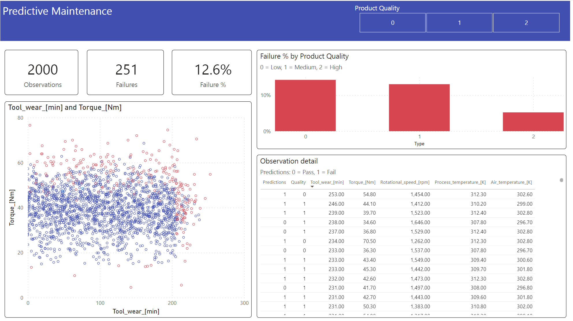
The dashboard shows that Tool_wear and Torque create a noticeable boundary between failed and unfailed cases, as expected from the earlier correlation analysis in step 2.