Übung: Schätzen von Ressourcen für ein reales Problem
Der Faktoringalgorithmus von Shor ist einer der bekanntesten Quantenalgorithmen. Er bietet eine exponentiell höhere Geschwindigkeit gegenüber jedem bekannten klassischen Faktoringalgorithmus.
Klassische Kryptografie verwendet physikalische oder mathematische Mittel wie rechnerische Schwierigkeiten, um eine Aufgabe zu erledigen. Ein beliebtes kryptografisches Protokoll ist das RSA-Schema (Rivest-Shamir-Adleman), das auf der Annahme der Schwierigkeit basiert, Primzahlen mithilfe eines klassischen Computers zu faktorisieren.
Der Algorithmus von Shor impliziert, dass Kryptografieverfahren mit öffentlichem Schlüssel von Quantencomputern geknackt werden können, wenn diese groß genug sind. Die Schätzung der für den Shor-Algorithmus erforderlichen Ressourcen ist wichtig, um das Sicherheitsrisiko dieser kryptografischen Schematypen zu bewerten.
In der folgenden Übung berechnen Sie die Ressourcenschätzungen für die Faktorisierung einer ganzen Zahl mit 2.048 Bit. Für diese Anwendung berechnen Sie die Schätzungen für die physischen Ressourcen direkt aus vorberechneten Schätzungen für die logischen Ressourcen. Für das tolerierte Fehlerbudget verwenden Sie $\epsilon = 1/3$.
Schreiben des Shor-Algorithmus
Wählen Sie in Visual Studio Code die Optionen Ansicht > Befehlspalette und dann Erstellen: Verwenden von Jupyter Notebook.
Speichern Sie das Notebook als ShorRE.ipynb.
Importieren Sie das
qsharp-Paket in der ersten Zelle.import qsharpVerwenden Sie den
Microsoft.Quantum.ResourceEstimation-Namespace, um eine zwischengespeicherte, optimierte Version des Ganzzahlfaktorisierungsalgorithmus von Shor zu definieren. Fügen Sie eine neue Zelle hinzu, kopieren Sie den folgenden Code, und fügen Sie ihn in die Zelle ein:%%qsharp open Microsoft.Quantum.Arrays; open Microsoft.Quantum.Canon; open Microsoft.Quantum.Convert; open Microsoft.Quantum.Diagnostics; open Microsoft.Quantum.Intrinsic; open Microsoft.Quantum.Math; open Microsoft.Quantum.Measurement; open Microsoft.Quantum.Unstable.Arithmetic; open Microsoft.Quantum.ResourceEstimation; operation RunProgram() : Unit { let bitsize = 31; // When choosing parameters for `EstimateFrequency`, make sure that // generator and modules are not co-prime let _ = EstimateFrequency(11, 2^bitsize - 1, bitsize); } // In this sample we concentrate on costing the `EstimateFrequency` // operation, which is the core quantum operation in Shors algorithm, and // we omit the classical pre- and post-processing. /// # Summary /// Estimates the frequency of a generator /// in the residue ring Z mod `modulus`. /// /// # Input /// ## generator /// The unsigned integer multiplicative order (period) /// of which is being estimated. Must be co-prime to `modulus`. /// ## modulus /// The modulus which defines the residue ring Z mod `modulus` /// in which the multiplicative order of `generator` is being estimated. /// ## bitsize /// Number of bits needed to represent the modulus. /// /// # Output /// The numerator k of dyadic fraction k/2^bitsPrecision /// approximating s/r. operation EstimateFrequency( generator : Int, modulus : Int, bitsize : Int ) : Int { mutable frequencyEstimate = 0; let bitsPrecision = 2 * bitsize + 1; // Allocate qubits for the superposition of eigenstates of // the oracle that is used in period finding. use eigenstateRegister = Qubit[bitsize]; // Initialize eigenstateRegister to 1, which is a superposition of // the eigenstates we are estimating the phases of. // We first interpret the register as encoding an unsigned integer // in little endian encoding. ApplyXorInPlace(1, eigenstateRegister); let oracle = ApplyOrderFindingOracle(generator, modulus, _, _); // Use phase estimation with a semiclassical Fourier transform to // estimate the frequency. use c = Qubit(); for idx in bitsPrecision - 1..-1..0 { within { H(c); } apply { // `BeginEstimateCaching` and `EndEstimateCaching` are the operations // exposed by Azure Quantum Resource Estimator. These will instruct // resource counting such that the if-block will be executed // only once, its resources will be cached, and appended in // every other iteration. if BeginEstimateCaching("ControlledOracle", SingleVariant()) { Controlled oracle([c], (1 <<< idx, eigenstateRegister)); EndEstimateCaching(); } R1Frac(frequencyEstimate, bitsPrecision - 1 - idx, c); } if MResetZ(c) == One { set frequencyEstimate += 1 <<< (bitsPrecision - 1 - idx); } } // Return all the qubits used for oracles eigenstate back to 0 state // using Microsoft.Quantum.Intrinsic.ResetAll. ResetAll(eigenstateRegister); return frequencyEstimate; } /// # Summary /// Interprets `target` as encoding unsigned little-endian integer k /// and performs transformation |k⟩ ↦ |gᵖ⋅k mod N ⟩ where /// p is `power`, g is `generator` and N is `modulus`. /// /// # Input /// ## generator /// The unsigned integer multiplicative order ( period ) /// of which is being estimated. Must be co-prime to `modulus`. /// ## modulus /// The modulus which defines the residue ring Z mod `modulus` /// in which the multiplicative order of `generator` is being estimated. /// ## power /// Power of `generator` by which `target` is multiplied. /// ## target /// Register interpreted as LittleEndian which is multiplied by /// given power of the generator. The multiplication is performed modulo /// `modulus`. internal operation ApplyOrderFindingOracle( generator : Int, modulus : Int, power : Int, target : Qubit[] ) : Unit is Adj + Ctl { // The oracle we use for order finding implements |x⟩ ↦ |x⋅a mod N⟩. We // also use `ExpModI` to compute a by which x must be multiplied. Also // note that we interpret target as unsigned integer in little-endian // encoding by using the `LittleEndian` type. ModularMultiplyByConstant(modulus, ExpModI(generator, power, modulus), target); } /// # Summary /// Performs modular in-place multiplication by a classical constant. /// /// # Description /// Given the classical constants `c` and `modulus`, and an input /// quantum register (as LittleEndian) |𝑦⟩, this operation /// computes `(c*x) % modulus` into |𝑦⟩. /// /// # Input /// ## modulus /// Modulus to use for modular multiplication /// ## c /// Constant by which to multiply |𝑦⟩ /// ## y /// Quantum register of target internal operation ModularMultiplyByConstant(modulus : Int, c : Int, y : Qubit[]) : Unit is Adj + Ctl { use qs = Qubit[Length(y)]; for (idx, yq) in Enumerated(y) { let shiftedC = (c <<< idx) % modulus; Controlled ModularAddConstant([yq], (modulus, shiftedC, qs)); } ApplyToEachCA(SWAP, Zipped(y, qs)); let invC = InverseModI(c, modulus); for (idx, yq) in Enumerated(y) { let shiftedC = (invC <<< idx) % modulus; Controlled ModularAddConstant([yq], (modulus, modulus - shiftedC, qs)); } } /// # Summary /// Performs modular in-place addition of a classical constant into a /// quantum register. /// /// # Description /// Given the classical constants `c` and `modulus`, and an input /// quantum register (as LittleEndian) |𝑦⟩, this operation /// computes `(x+c) % modulus` into |𝑦⟩. /// /// # Input /// ## modulus /// Modulus to use for modular addition /// ## c /// Constant to add to |𝑦⟩ /// ## y /// Quantum register of target internal operation ModularAddConstant(modulus : Int, c : Int, y : Qubit[]) : Unit is Adj + Ctl { body (...) { Controlled ModularAddConstant([], (modulus, c, y)); } controlled (ctrls, ...) { // We apply a custom strategy to control this operation instead of // letting the compiler create the controlled variant for us in which // the `Controlled` functor would be distributed over each operation // in the body. // // Here we can use some scratch memory to save ensure that at most one // control qubit is used for costly operations such as `AddConstant` // and `CompareGreaterThenOrEqualConstant`. if Length(ctrls) >= 2 { use control = Qubit(); within { Controlled X(ctrls, control); } apply { Controlled ModularAddConstant([control], (modulus, c, y)); } } else { use carry = Qubit(); Controlled AddConstant(ctrls, (c, y + [carry])); Controlled Adjoint AddConstant(ctrls, (modulus, y + [carry])); Controlled AddConstant([carry], (modulus, y)); Controlled CompareGreaterThanOrEqualConstant(ctrls, (c, y, carry)); } } } /// # Summary /// Performs in-place addition of a constant into a quantum register. /// /// # Description /// Given a non-empty quantum register |𝑦⟩ of length 𝑛+1 and a positive /// constant 𝑐 < 2ⁿ, computes |𝑦 + c⟩ into |𝑦⟩. /// /// # Input /// ## c /// Constant number to add to |𝑦⟩. /// ## y /// Quantum register of second summand and target; must not be empty. internal operation AddConstant(c : Int, y : Qubit[]) : Unit is Adj + Ctl { // We are using this version instead of the library version that is based // on Fourier angles to show an advantage of sparse simulation in this sample. let n = Length(y); Fact(n > 0, "Bit width must be at least 1"); Fact(c >= 0, "constant must not be negative"); Fact(c < 2 ^ n, $"constant must be smaller than {2L ^ n}"); if c != 0 { // If c has j trailing zeroes than the j least significant bits // of y will not be affected by the addition and can therefore be // ignored by applying the addition only to the other qubits and // shifting c accordingly. let j = NTrailingZeroes(c); use x = Qubit[n - j]; within { ApplyXorInPlace(c >>> j, x); } apply { IncByLE(x, y[j...]); } } } /// # Summary /// Performs greater-than-or-equals comparison to a constant. /// /// # Description /// Toggles output qubit `target` if and only if input register `x` /// is greater than or equal to `c`. /// /// # Input /// ## c /// Constant value for comparison. /// ## x /// Quantum register to compare against. /// ## target /// Target qubit for comparison result. /// /// # Reference /// This construction is described in [Lemma 3, arXiv:2201.10200] internal operation CompareGreaterThanOrEqualConstant(c : Int, x : Qubit[], target : Qubit) : Unit is Adj+Ctl { let bitWidth = Length(x); if c == 0 { X(target); } elif c >= 2 ^ bitWidth { // do nothing } elif c == 2 ^ (bitWidth - 1) { ApplyLowTCNOT(Tail(x), target); } else { // normalize constant let l = NTrailingZeroes(c); let cNormalized = c >>> l; let xNormalized = x[l...]; let bitWidthNormalized = Length(xNormalized); let gates = Rest(IntAsBoolArray(cNormalized, bitWidthNormalized)); use qs = Qubit[bitWidthNormalized - 1]; let cs1 = [Head(xNormalized)] + Most(qs); let cs2 = Rest(xNormalized); within { for i in IndexRange(gates) { (gates[i] ? ApplyAnd | ApplyOr)(cs1[i], cs2[i], qs[i]); } } apply { ApplyLowTCNOT(Tail(qs), target); } } } /// # Summary /// Internal operation used in the implementation of GreaterThanOrEqualConstant. internal operation ApplyOr(control1 : Qubit, control2 : Qubit, target : Qubit) : Unit is Adj { within { ApplyToEachA(X, [control1, control2]); } apply { ApplyAnd(control1, control2, target); X(target); } } internal operation ApplyAnd(control1 : Qubit, control2 : Qubit, target : Qubit) : Unit is Adj { body (...) { CCNOT(control1, control2, target); } adjoint (...) { H(target); if (M(target) == One) { X(target); CZ(control1, control2); } } } /// # Summary /// Returns the number of trailing zeroes of a number /// /// ## Example /// ```qsharp /// let zeroes = NTrailingZeroes(21); // = NTrailingZeroes(0b1101) = 0 /// let zeroes = NTrailingZeroes(20); // = NTrailingZeroes(0b1100) = 2 /// ``` internal function NTrailingZeroes(number : Int) : Int { mutable nZeroes = 0; mutable copy = number; while (copy % 2 == 0) { set nZeroes += 1; set copy /= 2; } return nZeroes; } /// # Summary /// An implementation for `CNOT` that when controlled using a single control uses /// a helper qubit and uses `ApplyAnd` to reduce the T-count to 4 instead of 7. internal operation ApplyLowTCNOT(a : Qubit, b : Qubit) : Unit is Adj+Ctl { body (...) { CNOT(a, b); } adjoint self; controlled (ctls, ...) { // In this application this operation is used in a way that // it is controlled by at most one qubit. Fact(Length(ctls) <= 1, "At most one control line allowed"); if IsEmpty(ctls) { CNOT(a, b); } else { use q = Qubit(); within { ApplyAnd(Head(ctls), a, q); } apply { CNOT(q, b); } } } controlled adjoint self; }
Schätzen des Algorithmus von Shor
Schätzen Sie nun die physischen Ressourcen für den RunProgram-Vorgang unter Verwendung der Standardannahmen. Fügen Sie eine neue Zelle hinzu, kopieren Sie den folgenden Code, und fügen Sie ihn in die Zelle ein:
result = qsharp.estimate("RunProgram()")
result
Eine qsharp.estimate-Funktion erstellt ein Ergebnisobjekt, mit dem Sie eine Tabelle mit der Gesamtanzahl der physischen Ressourcen anzeigen können. Sie können die Kostendetails einsehen, indem Sie die Gruppen, die mehr Informationen enthalten, zuklappen.
Reduzieren Sie beispielsweise die Gruppe der logischen Qubit-Parameter, um festzustellen, ob der Codeabstand 21 und die Anzahl der physischen Qubits 882 ist.
| Logischer Qubit-Parameter | Wert |
|---|---|
| QEC-Schema | surface_code |
| Codeabstand | 21 |
| Physische Qubits | 882 |
| Logische Zykluszeit | 8 Millisek. |
| Logische Qubit-Fehlerrate | 3.00E-13 |
| Crossing Prefactor | 0,03 |
| Schwellenwert für die Fehlerkorrektur | 0.01 |
| Formel für die logische Zykluszeit | (4 × twoQubitGateTime × 2 × oneQubitMeasurementTime) × codeDistance |
| Formel für physische Qubits | 2 × codeDistance * codeDistance |
Tipp
Für eine kompaktere Version der Ausgabetabelle können Sie result.summary verwenden.
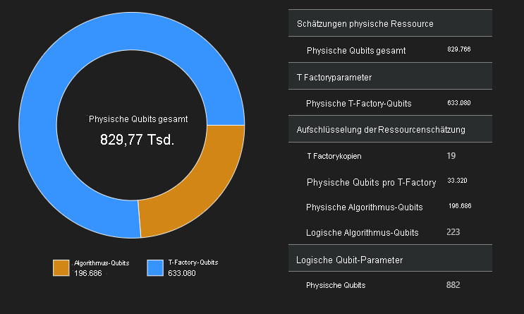
Raumdiagramm
Die Verteilung physischer Qubits, die für den Algorithmus und die T-Factorys verwendet werden, ist ein Faktor, der sich auf das Design Ihres Algorithmus auswirken kann. Sie können das qsharp-widgets-Paket verwenden, um diese Verteilung zu visualisieren, um die geschätzten Platzanforderungen des Algorithmus besser zu verstehen.
from qsharp_widgets import SpaceChart
SpaceChart(result)
In diesem Beispiel ist die Anzahl der zum Ausführen des Algorithmus erforderlichen physischen Qubits 829.766, von denen 196.686 Algorithmus-Qubits und 633.080 T-Factory-Qubits sind.
Vergleichen der Ressourcenschätzungen für verschiedene Qubit-Technologien
Mit Azure Quantum Resource Estimator können Sie mehrere Konfigurationen von Zielparametern ausführen und die Ergebnisse vergleichen. Dies ist nützlich, wenn Sie die Kosten verschiedener Qubit-Modelle, QEC-Schemas oder Fehlerbudgets vergleichen möchten.
Sie können auch eine Liste der Schätzungsparameter mithilfe des EstimatorParams-Objekts erstellen.
from qsharp.estimator import EstimatorParams, QubitParams, QECScheme, LogicalCounts

labels = ["Gate-based µs, 10⁻³", "Gate-based µs, 10⁻⁴", "Gate-based ns, 10⁻³", "Gate-based ns, 10⁻⁴", "Majorana ns, 10⁻⁴", "Majorana ns, 10⁻⁶"]

params = EstimatorParams(6)
params.error_budget = 0.333
params.items[0].qubit_params.name = QubitParams.GATE_US_E3
params.items[1].qubit_params.name = QubitParams.GATE_US_E4
params.items[2].qubit_params.name = QubitParams.GATE_NS_E3
params.items[3].qubit_params.name = QubitParams.GATE_NS_E4
params.items[4].qubit_params.name = QubitParams.MAJ_NS_E4
params.items[4].qec_scheme.name = QECScheme.FLOQUET_CODE
params.items[5].qubit_params.name = QubitParams.MAJ_NS_E6
params.items[5].qec_scheme.name = QECScheme.FLOQUET_CODE

qsharp.estimate("RunProgram()", params=params).summary_data_frame(labels=labels)
| Qubitmodell | Logische Qubits | Logische Tiefe | T-Zustände | Codeabstand | T-Factorys | T-Factoryanteil | Physische Qubits | rQOPS | Physische Ausführungszeit |
|---|---|---|---|---|---|---|---|---|---|
| Gatterbasiert µs, 10⁻³ | 223 3,64M | 4,70 M | 17 | 13 | 40,54 % | 216,77 k | 21,86 k | 10 Stunden | |
| Gatterbasiert µs, 10⁻⁴ | 223 | 3,64 M | 4,70 M | 9 | 14 | 43,17 % | 63,57 k | 41,30 k | 5 Stunden |
| Gatterbasiert ns, 10⁻³ | 223 3,64M | 4,70 M | 17 | 16 | 69,08 % | 416,89 k | 32,79 M | 25 Sek. | |
| Gatterbasiert ns, 10⁻⁴ | 223 3,64M | 4,70 M | 9 | 14 | 43,17 % | 63,57 k | 61,94 M | 13 Sek. | |
| Majorana ns, 10⁻⁴ | 223 3,64M | 4,70 M | 9 | 19 | 82,75 % | 501,48 k | 82,59 M | 10 Sek. | |
| Majorana ns, 10⁻⁶ | 223 3,64M | 4,70 M | 5 | 13 | 31,47 % | 42,96 k | 148,67 M | 5 s |
Extrahieren von Ressourcenschätzungen aus logischen Ressourcenzählungen
Wenn Sie bereits einige Schätzungen für einen Vorgang kennen, können Sie mit Resource Estimator die bekannten Schätzungen in die Gesamtkosten des Programms integrieren, um die Ausführungszeit zu reduzieren. Sie können die LogicalCounts-Klasse verwenden, um die logischen Ressourcenschätzungen aus vorab berechneten Ressourcenschätzwerten zu extrahieren.
Wählen Sie Code aus, um eine neue Zelle hinzuzufügen, und geben Sie dann den folgenden Code ein, und führen Sie diesen aus:
logical_counts = LogicalCounts({
    'numQubits': 12581,
    'tCount': 12,
    'rotationCount': 12,
    'rotationDepth': 12,
    'cczCount': 3731607428,
    'measurementCount': 1078154040})

logical_counts.estimate(params).summary_data_frame(labels=labels)
| Qubitmodell | Logische Qubits | Logische Tiefe | T-Zustände | Codeabstand | T-Factorys | T-Factoryanteil | Physische Qubits | Physische Ausführungszeit |
|---|---|---|---|---|---|---|---|---|
| Gatterbasiert µs, 10⁻³ | 25.481 | 1,2e+10 | 1,5e+10 | 27 | 13 | 0,6% | 37,38 Mio. | 6 Jahre |
| Gatterbasiert µs, 10⁻⁴ | 25.481 | 1,2e+10 | 1,5e+10 | 13 | 14 | 0,8 % | 8,68 Mio. | 3 Jahre |
| Gatterbasiert ns, 10⁻³ | 25.481 | 1,2e+10 | 1,5e+10 | 27 | 15 | 1,3 % | 37,65 Mio. | 2 Tage |
| Gatterbasiert ns, 10⁻⁴ | 25.481 | 1,2e+10 | 1,5e+10 | 13 | 18 | 1,2 % | 8,72 Mio. | 18 Stunden |
| Majorana ns, 10⁻⁴ | 25.481 | 1,2e+10 | 1,5e+10 | 15 | 15 | 1,3 % | 26,11 Mio. | 15 Stunden |
| Majorana ns, 10⁻⁶ | 25.481 | 1,2e+10 | 1,5e+10 | 7 | 13 | 0,5 % | 6,25 Mio. | 7 Stunden |
Zusammenfassung
Schlimmstenfalls würden Quantencomputer mit gatterbasierten μs-Qubits (Qubits mit Betriebszeiten im Nanosekundenregime wie supraleitende Qubits) und einem QEC-Oberflächencode sechs Jahre und 37,38 Millionen Qubits benötigen, um eine ganze Zahl mit 2,048 Bit mit dem Shor-Algorithmus zu faktorisieren.
Wenn Sie eine andere Qubit-Technologie, z. B. gatterbasierte ns-Ionen-Qubits, und denselben Oberflächencode verwenden, ändert sich die Anzahl der Qubits nicht viel, aber die Ausführungszeit beträgt im schlechtesten Fall zwei Tage und im besten Fall 18 Stunden. Wenn Sie die Qubittechnologie und den QEC-Code ändern, z. B. in Majorana-basierte Qubits, könnte das Faktorisieren einer ganzen Zahl mit 2.048 Bit mithilfe des Shor-Algorithmus und einem Array von 6,25 Millionen Qubits im besten Fall in Stunden erfolgen.
Aus diesem Experiment können Sie schließen, dass die Verwendung von Majorana-Qubits mit einem Floquet-QEC-Code die beste Wahl ist, um den Shor-Algorithmus auszuführen und 2,048-Bit-Integer zu faktorisieren.