Forecasting API overview
The Forecasting API, also known as the Time Series API, is designed to predict future values of a specific indicator based on its past, time-ordered observations. This API is useful for two reasons:
- The dataset required for training is simple – it primarily needs labels. Features aren't needed for forecasting. The only requirement is that values must be sorted chronologically and that they must represent the same time interval.
- Business applications are full of data, which is sorted chronologically. Approximately 30% of all tables contain a column of type Date and a column of type Decimal.
Forecasting Model
The Forecasting Model for Dynamics 365 Business Central lets you analyze data in historical periods to make predictions about cash flow and inventory levels. This model uses R code to calculate the forecast and determine accuracy.
Input Data Schema
The experiment uses historical time series values from the following fields:
- GranularityAttribute (String) - Can be associated with a product ID to forecast product sales. The Group ID can be a composite key that includes the product ID and a location ID or variant.
- DateKey (Numeric) - Ordinal number of time-periods, such as days, weeks, months, or years. The model expects the same duration for each period.
- TransactionQty (Numeric) - The forecast value for the quantity of items sold, total payables or receivables, or the percentage of capacity that was used.
Additionally, the model requires a set of parameters for modules:
- Horizon (Numeric) - Specifies the number of future periods to make predictions for.
- Seasonality (Numeric) – The model accepts any type of time-period, but if you want it to recognize seasonality you need to define what a normal season is for the historical data. For example, if the season is a year and the values are grouped monthly, then seasonality should be 12. If the season contains quarterly values, then seasonality should be 4. However, if seasonality in your business is weekly, use 7 and aggregate values daily.
- Forecast_start_datekey (Numeric) – Specifies a delay before forecasting starts. Here’s an example. Today is January 1, and your data is for the past year, which is 12 periods. You can enter 2 as the Horizon, and 15 for Forecast_start_datekey. In this case, you skip two months, and get predictions for March and April. You can achieve the same result by specifying 4 as the Horizon, and skipping the first 2 periods when processing the response. In this case, specify Forecast_start_datekey as the last value of DateKey field, and increment it by 1. For example, if you provide 12 months of historical data, and the last DateKey is 12, the Forecast_start_datekey is 13 (12+1).
- Time_series_model (String) - Specifies the time series model to use. The model supports the following algorithms, and combinations of them:
- ARIMA
- ETS
- STL
- ETS+ARIMA (returns average as result)
- ETS+STL (returns average as result)
- ALL
- TBATS
If you choose ALL the model compares the results and returns the one that has the lowest mean absolute percentage error (MAPE).
- Confidence_level (Numeric) - In the model output, notice that in addition to the forecasted value, the model also returns the sigma, or variance. This is the range that future values are predicted to fall within, with the probability defined by the confidence level. So, if the confidence level is 95%, the forecasted value might be 100, for example, and the sigma 20. This means that with a probability of 95%, the actual value is somewhere in between 80 and 120 (100+/-20). If you set the confidence_level to 85, the sigma is lower. In the previous example, it can be that the forecasted value is 100 and the sigma 14. Together, this means that, with a probability of 85%, the actual value is somewhere between 86 and 114.
Output Data Schema
The output of the service shows the calculated forecast values with confidence levels in the following fields:
- GranularityAttribute (String) - Can be associated with a product ID to forecast product sales.
- The DateKey (Numeric) field – Ordinal number of the forecasted time-period. For example, if you provide 12 months of historical data, and the last DateKey is 12, and the horizon is 3, the model returns three sequential DateKey values, 13, 14 and 15, for each GranularityAttribute.
- The TransactionQty (Numeric) – The forecast value for the quantity of items sold, total payables or receivables, or the percentage of capacity that was used.
- The Sigma (Numeric) – Specifies the range that the forecast values are expected to fall within. This indicates the quality of predictions. For example, if TransactionQty is 100, and Sigma is 10, the forecast value is somewhere between 90 and 110. This is a good prediction. If Sigma is 100, however, the forecast value is between 0 and 200, which isn't a reliable prediction.
Forecasting API
All logic of the Forecasting API is encapsulated in the Time Series Management codeunit (ID 2000) and it consists of the following methods:
For Business Central online, the experiment is published by Microsoft and connected to the Microsoft subscription. For other deployment options, you have to create Machine Learning resources in your own Azure subscription. You can find sample steps in the sample repo.
The purpose of this task is to get the API URI and API key and pass them into the Initialize method. That gives the Forecasting API the end-point to contact:
var
  TimeSeriesManagement: Codeunit "Time Series Management";
  URITxt: TextConst ENU = 'https://..f1e/execute?api-version=2.0&details=true';
  KeyTxt: TextConst ENU = '1MhwM1T..oF4U2A==';
begin
  TimeSeriesManagement.Initialize(URITxt, KeyTxt, 0, false);
If you pass empty strings, the system uses the default end-point, but that only works for Business Central online:
TimeSeriesManagement.Initialize('', '', 0, true);
Once initialized, you must prepare the training dataset. There are two options:
- You can prepare the dataset "manually” by inserting records into a temporary instance of the Time Series Buffer table.
- Or, you can use the helper method
PrepareData, which do it for you. ThePrepareDatamethod transforms any passed record into a format, which can be processed by the Forecasting API. For example, if you want to detect sales volume, you'll probably use the Item Ledger Entry table as the source table:
var
  ItemLedgerEntry: Record "Item Ledger Entry";
  Date: Record Date;
begin
  ItemLedgerEntry.Reset();
  ItemLedgerEntry.SetRange("Entry Type", ItemLedgerEntry."Entry Type"::Sale);
  TimeSeriesManagement.PrepareData(
    ItemLedgerEntry,			                    //Source record
    ItemLedgerEntry.FieldNo("Item No."),	    //Field for grouping
    ItemLedgerEntry.FieldNo("Posting Date"),	//Date field
    ItemLedgerEntry.FieldNo(Quantity),	      //Aggregation field
    Date."Period Type"::Month, 		            //Period representing 1 data point
    WorkDate(), 			                        //Forecasting Start Date
    12);				                              //Number of data points
The provided code prepares the Item Ledger Entry table by filtering it by the Entry Type field because we need to focus on sales transactions. Then, we must specify, which field should be used for chronological ordering of dataset. There could be multiple fields, such as Posting Date and Document Date, so we need to specify, which field to be used for processing.
The Period Type field specifies how to aggregate transactions. Notice that the Forecasting API requires data points separated by the same interval, which can be day, week, month, quarter, or even year. It all depends on the amount of available data and a reasonable interval for prediction.
The number of data points specifies how many data points must be produced by the method.
Note
The Forecasting API doesn’t tolerate missing data points. If you have 0 sales on Monday and 3 on Tuesday, you still need to report one value for Monday (0) and one for Tuesday (the sum of 3 separate transactions).
The method aggregates data, starting from the specified date and will move backwards. In this example, the method returns aggregated sales for 12 months preceding the work date.
Most probably your Item Ledger Entry table contains information about multiple items. The Forecasting API supports bulk processing, so you get a forecast for multiple entries. In this example, we use “Item No.” as the grouping field, so the PrepareData method prepares a dataset for each item.
You can read the prepared dataset with the GetPreparedData method.
var
  TempTimeSeriesBuffer: Record "Time Series Buffer" temporary;
begin
  TimeSeriesManagement.GetPreparedData(TempTimeSeriesBuffer);
If you create a page based on the Time Series Buffer table, you can display the training dataset for inspection:
| Group ID | Period No. | Period Start Date | Value |
|---|---|---|---|
| 1896-S | 1 | April, YYYY | -10.00 |
| 1896-S | 2 | May, YYYY | -6.00 |
| 1896-S | 3 | June, YYYY | -8.00 |
| 1896-S | 4 | July, YYYY | -9.00 |
| 1896-S | 5 | August, YYYY | -9.00 |
| 1896-S | 6 | September, YYYY | -11.00 |
| 1896-S | 7 | October, YYYY | -10.00 |
| 1896-S | 8 | November, YYYY | -15.00 |
| 1896-S | 9 | December, YYYY | -14.00 |
| 1896-S | 10 | January, YYYY+1 | -18.00 |
| 1896-S | 11 | February, YYYY+1 | -15.00 |
| 1896-S | 12 | March, YYYY+1 | -13.00 |
You can see 12 periods for each item (only one item is displayed on screenshot).
You can update the dataset (for example invert the sign for values) or create your own dataset if you need to collect data from more than one table. Then, you can send that dataset back to the Forecasting API with the SetPreparedData method. That's what we do with the Cash Flow Forecast, where we gather data from the Customer Ledger Entries, Vendor Ledger Entries, and Tax Entries tables.
Once your dataset is ready, it's time to run the Forecast method. The only parameter you need to specify is the number of data points that you want to forecast:
TimeSeriesManagement.Forecast(3, 0, 0);
The quality of the forecast is affected by specifying too many data points at a time. We address that later in this article.
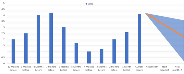
Now, you can get results for further processing. The GetForecast method fills the Time Series Forecast table with results.
    var
        TempTimeSeriesForecast: Record "Time Series Forecast" temporary;
    begin
        TimeSeriesManagement.GetForecast(TempTimeSeriesForecast);
The following image shows the forecast for the next 3 periods (13, 14, 15) that comes after the initial 12. There are forecasted values and delta for each data point.
| Group ID | Period No. | Period Start Date | Value | Delta | Delta % |
|---|---|---|---|---|---|
| 1896-S | 13 | April, YYYY+1 | -13.00 | 3.48 | 26.75 |
| 1896-S | 14 | May, YYYY+1 | -13.00 | 4.92 | 37.83 |
| 1896-S | 15 | June, YYYY+1 | -13.00 | 6.02 | 46.33 |
The Forecasting API doesn’t return the single value for a data point, but returns a range where the predicted value will be. In the example above, the period 15 has a predicted value of 13 and a delta of 6.02. This means that the value for the 15th period will be somewhere between 6.98 and 19.02 (13-6.02 and 13+6.02). Depending on what you're predicting, it might be good to ignore forecasts where the delta is wider than 20-30%. The narrower the better.
Fine-tuning the results
The experiment accepts many parameters to fine-tune results. Not all parameters are exposed in the API, but the Time Series Model is, and it accepts the following options that represent various time series algorithms and their combinations:
- ARIMA
- ETS
- STL
- ETS+ARIMA (returns average as a result)
- ETS+STL (returns average as a result)
- TBATS
- ALL
When you run the TimeSeriesManagement.Forecast(3, 0, 0); the ARIMA model is used for calculation. It’s usually a good choice to start with, but which model to choose, depends on the data that you have.
Let’s run all possible options and compare the results. In AL, define the enum as shown below:
enum 50139 "Time Series Model"
{
    value(0; ARIMA) { }
    value(1; ETS) { }
    value(2; STL) { }
    value(3; ETS_ARIMA) { Caption = 'ETS+ARIMA'; }
    value(4; ETS_STL) { Caption = 'ETS+STL'; }
    value(5; ALL) { }
    value(6; TBATS) { }
}
And then run the code that we wrote in the previous section, now with a different value for the Model parameter.
var
  TimeSeriesModel: enum "Time Series Model";
begin
  TimeSeriesManagement.Forecast(3, 0, TimeSeriesModel::ARIMA);
If you modify this code to run in a loop, you can get the following result:
| Group ID | Period No. | Period Start Date | Value | Delta | Delta % |
|---|---|---|---|---|---|
| ALL | 13 | April, YYYY+1 | -8.00 | 0,00037 | 0.00 |
| ALL | 14 | May, YYYY+1 | -4.00 | 0,00052 | 0.01 |
| ALL | 15 | June, YYYY+1 | -5.00 | 0,00064 | 0.01 |
| ARIMA | 13 | April, YYYY+1 | -16.95 | 3,98516 | 23.50 |
| ARIMA | 14 | May, YYYY+1 | -16.18 | 4,96880 | 30.72 |
| ARIMA | 15 | June, YYYY+1 | -15.60 | 5,43814 | 24.87 |
| ETS | 13 | April, YYYY+1 | -18.00 | 3,73638 | 20.76 |
| ETS | 14 | May, YYYY+1 | -18.00 | 5,28378 | 29.35 |
| ETS | 15 | June, YYYY+1 | -18.00 | 6,47117 | 35.95 |
| ETS+ARIMA | 13 | April, YYYY+1 | -17.48 | 2,73139 | 15.63 |
| ETS+ARIMA | 14 | May, YYYY+1 | -17.09 | 3,62654 | 21.22 |
| ETS+ARIMA | 15 | June, YYYY+1 | -16.80 | 4,22639 | 25.16 |
| TBATS | 13 | April, YYYY+1 | -8.00 | 0,00037 | 0.00 |
| TBATS | 14 | May, YYYY+1 | -4.00 | 0,00052 | 0.01 |
| TBATS | 15 | June, YYYY+1 | -5.00 | 0,00064 | 0.01 |
Based on this output, there are two major observations:
- The ALL model displays same result as the TBATS model. When you choose ALL as the option, it runs all available algorithms, compares the results, and returns the one that has the lowest, absolute percentage error (MAPE). For this dataset that appears to be the TBATS model.
- We also notice that the STL and STL+ETS models are missing. That’s because STL is an acronym for a seasonal decomposition of time series by Loess, and it focuses on seasonality. In the Forecasting API, the season is specified as one year. STL requires data for more than two years.
Let’s try to run the same code but with data for 26 months.
| Group ID | Period No. | Period Start Date | Value | Delta | Delta % |
|---|---|---|---|---|---|
| ALL | 27 | April, YYYY+1 | -20.06 | 1,76106 | 8.78 |
| ALL | 28 | May, YYYY+1 | -19.44 | 2,38266 | 12.26 |
| ALL | 29 | June, YYYY+1 | -19.10 | 2,90400 | 15.20 |
| ARIMA | 27 | April, YYYY+1 | -18.00 | 3,73193 | 20.73 |
| ARIMA | 28 | May, YYYY+1 | -18.00 | 5,27775 | 29.32 |
| ARIMA | 29 | June, YYYY+1 | -18.00 | 6,46390 | 35.91 |
| ETS | 27 | April, YYYY+1 | -18.00 | 3,65955 | 20.33 |
| ETS | 28 | May, YYYY+1 | -18.00 | 5,17513 | 28.75 |
| ETS | 29 | June, YYYY+1 | -18.00 | 6,33810 | 35.21 |
| ETS+ARIMA | 27 | April, YYYY+1 | -18.00 | 2,61341 | 14.52 |
| ETS+ARIMA | 28 | May, YYYY+1 | -18.00 | 3,69583 | 20.53 |
| ETS+ARIMA | 29 | June, YYYY+1 | -18.00 | 4,52641 | 25.15 |
| 27 | April, YYYY+1 | -17.91 | 2,00712 | 11.21 | |
| 28 | May, YYYY+1 | -16.54 | 2,84754 | 17.22 | |
| 29 | June, YYYY+1 | -16.56 | 3,54059 | 21.38 | |
| 27 | April, YYYY+1 | -17.81 | 1,64979 | 9.26 | |
| 28 | May, YYYY+1 | -15.07 | 2,37740 | 15.77 | |
| 29 | June, YYYY+1 | -15.11 | 3,15776 | 20.89 | |
| TBATS | 27 | April, YYYY+1 | -20.06 | 1,76106 | 8.78 |
| TBATS | 28 | May, YYYY+1 | -19.44 | 2,38266 | 12.26 |
| TBATS | 29 | June, YYYY+1 | -19.10 | 2,90400 | 15.20 |
Now, the STL and ETS+STL models are also capable of producing results. Notice that TBATS is still the best option. If so, why don’t we always use the TBATS model? Because it doesn’t work well on small datasets. Let’s rerun the same code for a dataset that contains six months only.
| Group ID | Period No. | Period Start Date | Value | Delta | Delta % |
|---|---|---|---|---|---|
| ALL | 7 | April, YYYY+1 | -17.26 | 0,00000 | 0.00 |
| ALL | 8 | May, YYYY+1 | -16.96 | 0,00000 | 0.00 |
| ALL | 9 | June, YYYY+1 | -20.32 | 0,00000 | 0.00 |
| 7 | April, YYYY+1 | -17.26 | 0,00000 | 0.00 | |
| 8 | May, YYYY+1 | -16.96 | 0,00000 | 0.00 | |
| 9 | June, YYYY+1 | -20.32 | 0,00000 | 0.00 | |
| ETS | 7 | April, YYYY+1 | -18.00 | 3,88030 | 21.56 |
| ETS | 8 | May, YYYY+1 | -18.00 | 5,48729 | 30.49 |
| ETS | 9 | June, YYYY+1 | -18.00 | 6,72042 | 37.34 |
| ETS+ARIMA | 7 | April, YYYY+1 | -17.63 | 0,00000 | 0.00 |
| ETS+ARIMA | 8 | May, YYYY+1 | -17.48 | 0,00000 | 0.00 |
| ETS+ARIMA | 9 | June, YYYY+1 | -19.16 | 0,00000 | 0.00 |
| TBATS | 7 | April, YYYY+1 | -29.20 | 0,00052 | 0.00 |
| TBATS | 8 | May, YYYY+1 | -66.98 | 0,00074 | 0.00 |
| TBATS | 9 | June, YYYY+1 | -140.35 | 0,00090 | 0.00 |
In the example, we see another two interesting facts:
- The amount of data didn’t allow the Forecasting API to calculate the range for the ARIMA model.
- Despite that, the ARIMA model is the best performer on this dataset. In contrast, TBATS returns extreme numbers.
What about always using ALL? That’s a good option, however with its own drawbacks:
- We've seen issues (timeouts) for the ARIMA model with larger datasets that contained more than 200 data points. As ALL will try to perform a calculation for all models including ARIMA, it encounters similar issues. The solution is to reduce the dataset, use specific models, and adjust the R script if you're using your own deployment of the machine learning R code.
- There are also some cost considerations to make. Running all models is often more expensive than running a specific one, as it requires more compute power.
For more information, see the source code of the Sales and Inventory Forecast extension. Alternatively, you can also take a closer look at the Cash Flow Forecast feature, which is part of the Base Application extension.
See also
Prediction API overview
The Sales and Inventory Forecast Extension
Analyzing Cash Flow in Your Company
Feedback
Coming soon: Throughout 2024 we will be phasing out GitHub Issues as the feedback mechanism for content and replacing it with a new feedback system. For more information see: https://aka.ms/ContentUserFeedback.
Submit and view feedback for