Exercise - Build Machine Learning Model - Training

15 minutes

To create a machine learning model, you need two datasets: one for training and one for testing. In practice, you often have only one dataset, so you split it into two. In this exercise, you will perform an 80-20 split on the DataFrame you prepared in the previous lab so you can use it to train a machine learning model. You will also separate the DataFrame into feature columns and label columns. The former contains the columns used as input to the model (for example, the flight's origin and destination and the scheduled departure time), while the latter contains the column that the model will attempt to predict — in this case, the ARR_DEL15 column, which indicates whether a flight will arrive on time.

Switch back to the Azure notebook that you created in the previous section. If you closed the notebook, you can sign back into the Microsoft Azure Notebooks portal, open your notebook, and use the Cell -> Run All to rerun the all of the cells in the notebook after opening it.
In a new cell at the end of the notebook, enter and execute the following statements:
```
from sklearn.model_selection import train_test_split
train_x, test_x, train_y, test_y = train_test_split(df.drop('ARR_DEL15', axis=1), df['ARR_DEL15'], test_size=0.2, random_state=42)
```
The first statement imports scikit-learn's train_test_split helper function. The second line uses the function to split the DataFrame into a training set containing 80% of the original data, and a test set containing the remaining 20%. The random_state parameter seeds the random-number generator used to do the splitting, while the first and second parameters are DataFrames containing the feature columns and the label column.
train_test_split returns four DataFrames. Use the following command to display the number of rows and columns in the DataFrame containing the feature columns used for training:
```
train_x.shape
```
Now use this command to display the number of rows and columns in the DataFrame containing the feature columns used for testing:
```
test_x.shape
```
How do the two outputs differ, and why?

Can you predict what you would see if you called shape on the other two DataFrames, train_y and test_y? If you're not sure, try it and find out.

There are many types of machine learning models. One of the most common is the regression model, which uses one of a number of regression algorithms to produce a numeric value — for example, a person's age or the probability that a credit-card transaction is fraudulent. You'll train a classification model, which seeks to resolve a set of inputs into one of a set of known outputs. A classic example of a classification model is one that examines e-mails and classifies them as "spam" or "not spam." Your model will be a binary classification model that predicts whether a flight will arrive on-time or late ("binary" because there are only two possible outputs).

One of the benefits of using scikit-learn is that you don't have to build these models — or implement the algorithms that they use — by hand. Scikit-learn includes a variety of classes for implementing common machine learning models. One of them is RandomForestClassifier, which fits multiple decision trees to the data and uses averaging to boost the overall accuracy and limit overfitting.

Execute the following code in a new cell to create a RandomForestClassifier object and train it by calling the fit method.
```
from sklearn.ensemble import RandomForestClassifier

model = RandomForestClassifier(random_state=13)
model.fit(train_x, train_y)
```
The output shows the parameters used in the classifier, including n_estimators, which specifies the number of trees in each decision-tree forest, and max_depth, which specifies the maximum depth of the decision trees. The values shown are the defaults, but you can override any of them when creating the RandomForestClassifier object.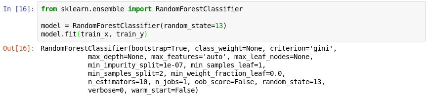

Training the model
Now call the predict method to test the model using the values in test_x, followed by the score method to determine the mean accuracy of the model:
```
predicted = model.predict(test_x)
model.score(test_x, test_y)
```
Confirm that you see the following output:

Testing the model

The mean accuracy is 86%, which seems good on the surface. However, mean accuracy isn't always a reliable indicator of the accuracy of a classification model. Let's dig a little deeper and determine how accurate the model really is — that is, how adept it is at determining whether a flight will arrive on time.

There are several ways to measure the accuracy of a classification model. One of the best overall measures for a binary classification model is Area Under Receiver Operating Characteristic Curve (sometimes referred to as "ROC AUC"), which essentially quantifies how often the model will make a correct prediction regardless of the outcome. In this unit, you'll compute an ROC AUC score for the model you built previously and learn about some of the reasons why that score is lower than the mean accuracy output by the score method. You'll also learn about other ways to gauge the accuracy of the model.

Before you compute the ROC AUC, you must generate prediction probabilities for the test set. These probabilities are estimates for each of the classes, or answers, the model can predict. For example, [0.88199435, 0.11800565] means that there's an 89% chance that a flight will arrive on time (ARR_DEL15 = 0) and a 12% chance that it won't (ARR_DEL15 = 1). The sum of the two probabilities adds up to 100%.

Run the following code to generate a set of prediction probabilities from the test data:
```
from sklearn.metrics import roc_auc_score
probabilities = model.predict_proba(test_x)
```
Now use the following statement to generate an ROC AUC score from the probabilities using scikit-learn's roc_auc_score method:
```
roc_auc_score(test_y, probabilities[:, 1])
```
Confirm that the output shows a score of 67%:

Generating an AUC score

Why is the AUC score lower than the mean accuracy computed in the previous exercise?

The output from the score method reflects how many of the items in the test set the model predicted correctly. This score is skewed by the fact that the dataset the model was trained and tested with contains many more rows representing on-time arrivals than rows representing late arrivals. Because of this imbalance in the data, you're more likely to be correct if you predict that a flight will be on time than if you predict that a flight will be late.

ROC AUC takes this into account and provides a more accurate indication of how likely it is that a prediction of on-time or late will be correct.
You can learn more about the model's behavior by generating a confusion matrix, also known as an error matrix. The confusion matrix quantifies the number of times each answer was classified correctly or incorrectly. Specifically, it quantifies the number of false positives, false negatives, true positives, and true negatives. This is important, because if a binary classification model trained to recognize cats and dogs is tested with a dataset that is 95% dogs, it could score 95% simply by guessing "dog" every time. But if it failed to identify cats at all, it would be of little value.

Use the following code to produce a confusion matrix for your model:
```
from sklearn.metrics import confusion_matrix
confusion_matrix(test_y, predicted)
```
The first row in the output represents flights that were on time. The first column in that row shows how many flights were correctly predicted to be on time, while the second column reveals how many flights were predicted as delayed but weren't. From this, the model appears to be adept at predicting that a flight will be on time.

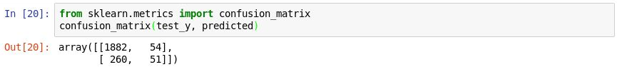
Generating a confusion matrix

But look at the second row, which represents flights that were delayed. The first column shows how many delayed flights were incorrectly predicted to be on time. The second column shows how many flights were correctly predicted to be delayed. Clearly, the model isn't nearly as adept at predicting that a flight will be delayed as it is at predicting that a flight will arrive on time. What you want in a confusion matrix is large numbers in the upper-left and lower-right corners, and small numbers (preferably zeros) in the upper-right and lower-left corners.
Other measures of accuracy for a classification model include precision and recall. Suppose the model was presented with three on-time arrivals and three delayed arrivals, and that it correctly predicted two of the on-time arrivals, but incorrectly predicted that two of the delayed arrivals would be on time. In this case, the precision would be 50% (two of the four flights it classified as being on time actually were on time), while its recall would be 67% (it correctly identified two of the three on-time arrivals). You can learn more about precision and recall from https://en.wikipedia.org/wiki/Precision_and_recall

Scikit-learn contains a handy method named precision_score for computing precision. To quantify the precision of your model, execute the following statements:
```
from sklearn.metrics import precision_score

train_predictions = model.predict(train_x)
precision_score(train_y, train_predictions)
```
Examine the output. What is your model's precision?

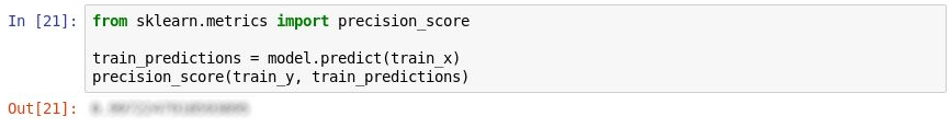
Measuring precision
Scikit-learn also contains a method named recall_score for computing recall. To measure you model's recall, execute the following statements:
```
from sklearn.metrics import recall_score

recall_score(train_y, train_predictions)
```
What is the model's recall?

Measuring recall
Use the File -> Save and Checkpoint command to save the notebook.

In the real world, a trained data scientist would look for ways to make the model even more accurate. Among other things, they would try different algorithms and take steps to tune the chosen algorithm to find the optimum combination of parameters. Another likely step would be to expand the dataset to millions of rows rather than a few thousand and also attempt to reduce the imbalance between late and on-time arrivals. But for our purposes, the model is fine as-is.

Continue

Exercise - Build Machine Learning Model

Feedback