Events
Power BI DataViz World Championships
14 Feb, 16 - 31 Mar, 16
With 4 chances to enter, you could win a conference package and make it to the LIVE Grand Finale in Las Vegas
Learn moreThis browser is no longer supported.
Upgrade to Microsoft Edge to take advantage of the latest features, security updates, and technical support.
This article targets data modelers who develop Power BI composite models. It describes composite model use cases, and provides you with design guidance. Specifically, the guidance can help you determine whether a composite model is appropriate for your solution. If it is, then this article will also help you design optimal composite models and reports.
Note
An introduction to composite models isn't covered in this article. If you're not completely familiar with composite models, we recommend that you first read the Use composite models in Power BI Desktop article.
Because composite models consist of at least one DirectQuery source, it's also important that you have a thorough understanding of model relationships, DirectQuery models, and DirectQuery model design guidance.
By definition, a composite model combines multiple source groups. A source group can represent imported data or a connection to a DirectQuery source. A DirectQuery source can be either a relational database or another tabular model, which can be a Power BI semantic model or an Analysis Services tabular model. When a tabular model connects to another tabular model, it's known as chaining. For more information, see Use composite models in Power BI Desktop.
Note
When a model connects to a tabular model but doesn't extend it with additional data, it's not a composite model. In this case, it's a DirectQuery model that connects to a remote model—so it comprises just the one source group. You might create this type of model to modify source model object properties, like a table name, column sort order, format string, or others.
Connecting to tabular models is especially relevant when extending an enterprise semantic model (when it's a Power BI semantic model or Analysis Services model). An enterprise semantic model is fundamental to the development and operation of a data warehouse. It provides an abstraction layer over the data in the data warehouse to present business definitions and terminology. It's commonly used as a link between physical data models and reporting tools, like Power BI. In most organizations, it's managed by a central team, and that's why it's described as enterprise. For more information, see the enterprise BI usage scenario.
You can consider developing a composite model in the following situations:
Note
Composite models can't include connections to certain external analytic databases. These databases include SAP Business Warehouse, and SAP HANA when treating SAP HANA as a multidimensional source.
While Power BI composite models can solve particular design challenges, they can contribute to slow performance. Also, in some situations, unexpected calculation results can occur (described later in this article). For these reasons, evaluate other model design options when they exist.
Whenever possible, it's best to develop a model in import mode. This mode provides the greatest design flexibility, and best performance. However, challenges related to large data volumes, or reporting on near real-time data, can't always be solved by import models. In either of these cases, you can consider a DirectQuery model, providing your data is stored in a single data source that's supported by DirectQuery mode. For more information, see DirectQuery models in Power BI Desktop.
Tip
If your objective is only to extend an existing tabular model with more data, whenever possible, add that data to the existing data source.
In a composite model, you can set the storage mode for each table (except calculated tables).
There are several possible scenarios when Power BI queries a composite model.
In summary, we recommend that you:
You can add user-defined aggregations to DirectQuery tables. Their purpose is to improve performance for higher grain queries.
When aggregations are cached in the model, they behave as import tables (although they can't be used like a model table). Adding import aggregations to a DirectQuery model will result in a composite model.
Note
Hybrid tables don't support aggregations because some of the partitions operate in import mode. It's not possible to add aggregations at the level of an individual DirectQuery partition.
We recommend that an aggregation follows a basic rule: Its row count should be at least a factor of 10 smaller than the underlying table. For example, if the underlying table stores 1 billion rows, then the aggregation table shouldn't exceed 100 million rows. This rule ensures that there's an adequate performance gain relative to the cost of creating and maintaining the aggregation.
When a model relationship spans source groups, it's known as a cross source group relationship. Cross source group relationships are also limited relationships because there's no guaranteed "one" side. For more information, see Relationship evaluation.
Note
In some situations, you can avoid creating a cross source group relationship. See the Use Sync slicers topic later in this article.
When defining cross source group relationships, consider the following recommendations.
Warning
Because Power BI Desktop doesn't thoroughly validate cross source group relationships, it's possible to create ambiguous relationships.
Consider a scenario of a complex relationship design and how it could produce different—yet valid—results.
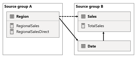
In this scenario, the Region table in source group A has a relationship to the Date table and Sales table in source group B. The relationship between the Region table and the Date table is active, while the relationship between the Region table and the Sales table is inactive. Also, there's an active relationship between the Region table and the Sales table, both of which are in source group B. The Sales table includes a measure named TotalSales, and the Region table includes two measures named RegionalSales and RegionalSalesDirect.
Here are the measure definitions.
TotalSales = SUM(Sales[Sales])
RegionalSales = CALCULATE([TotalSales], USERELATIONSHIP(Region[RegionID], Sales[RegionID]))
RegionalSalesDirect = CALCULATE(SUM(Sales[Sales]), USERELATIONSHIP(Region[RegionID], Sales[RegionID]))
Notice how the RegionalSales measure refers to the TotalSales measure, while the RegionalSalesDirect measure doesn't. Instead, the RegionalSalesDirect measure uses the expression SUM(Sales[Sales]), which is the expression of the TotalSales measure.
The difference in the result is subtle. When Power BI evaluates the RegionalSales measure, it applies the filter from the Region table to both the Sales table and the Date table. Therefore, the filter also propagates from the Date table to the Sales table. In contrast, when Power BI evaluates the RegionalSalesDirect measure, it only propagates the filter from the Region table to the Sales table. The results returned by RegionalSales measure and the RegionalSalesDirect measure could differ, even though the expressions are semantically equivalent.
Important
Whenever you use the CALCULATE function with an expression that's a measure in a remote source group, test the calculation results thoroughly.
Consider a scenario when a cross source group relationship has high-cardinality relationship columns.
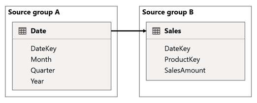
In this scenario, the Date table is related to the Sales table on the DateKey columns. The data type of the DateKey columns is integer, storing whole numbers that use the yyyymmdd format. The tables belong to different source groups. Further, it's a high-cardinality relationship because the earliest date in the Date table is January 1, 1900 and the latest date is December 31, 2100—so there's a total of 73,414 rows in the table (one row for each date in the 1900-2100 time span).
There are two cases for concern.
First, when you use the Date table columns as filters, filter propagation will filter the DateKey column of the Sales table to evaluate measures. When filtering by a single year, like 2022, the DAX query will include a filter expression like Sales[DateKey] IN { 20220101, 20220102, …20221231 }. The text size of the query can grow to become extremely large when the number of values in the filter expression is large, or when the filter values are long strings. It's expensive for Power BI to generate the long query and for the data source to run the query.
Second, when you use Date table columns—like Year, Quarter, or Month—as grouping columns, it results in filters that include all unique combinations of year, quarter, or month, and the DateKey column values. The string size of the query, which contains filters on the grouping columns and the relationship column, can become extremely large. That's especially true when the number of grouping columns and/or the cardinality of the join column (the DateKey column) is large.
To address any performance issues, you can:
Date table to the data source, resulting in a single source group model (meaning, it's no longer a composite model).MonthKey column to both tables and create the relationship on those columns. However, by raising the granularity of the relationship, you lose the ability to report on daily sales activity (unless you use the DateKey column from the Sales table).Consider a scenario when there aren't matching values between tables in a cross source group relationship.
In this scenario, the Date table in source group B has a relationship to the Sales table in that source group, and also to the Target table in source group A. All relationships are one-to-many from the Date table relating the Year columns. The Sales table includes a SalesAmount column that stores sales amounts, while the Target table includes a TargetAmount column that stores target amounts.
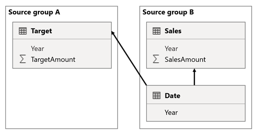
The Date table stores the years 2021 and 2022. The Sales table stores sales amounts for years 2021 (100) and 2022 (200), while the Target table stores target amounts for 2021 (100), 2022 (200), and 2023 (300)—a future year.

When a Power BI table visual queries the composite model by grouping on the Year column from the Date table and summing the SalesAmount and TargetAmount columns, it won't show a target amount for 2023. That's because the cross source group relationship is a limited relationship, and so it uses INNER JOIN semantics, which eliminate rows where there's no matching value on both sides. It will, however, produce a correct target amount total (600), because a Date table filter doesn't apply to its evaluation.
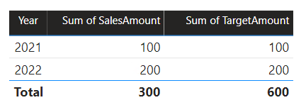
If the relationship between the Date table and the Target table is an intra source group relationship (assuming the Target table belonged to source group B), the visual will include a (Blank) year to show the 2023 (and any other unmatched years) target amount.
Important
To avoid misreporting, ensure that there are matching values in the relationship columns when dimension and fact tables reside in different source groups.
For more information about limited relationships, see Relationship evaluation.
You should consider specific limitations when adding calculated columns and calculation groups to a composite model.
Calculated columns added to a DirectQuery table that source their data from a relational database, like Microsoft SQL Server, are limited to expressions that operate on a single row at a time. These expressions can't use DAX iterator functions, like SUMX, or filter context modification functions, like CALCULATE.
Note
It's not possible to add calculated columns or calculated tables that depend on chained tabular models.
A calculated column expression on a remote DirectQuery table is limited to intra-row evaluation only. However, you can author such an expression, but it will result in an error when it's used in a visual. For example, if you add a calculated column to a remote DirectQuery table named DimProduct by using the expression [Product Sales] / SUM (DimProduct[ProductSales]), you'll be able to successfully save the expression in the model. However, it will result in an error when it's used in a visual because it violates the intra-row evaluation restriction.
In contrast, calculated columns added to a remote DirectQuery table that's a tabular model, which is either a Power BI semantic model or Analysis Services model, are more flexible. In this case, all DAX functions are allowed because the expression will be evaluated within the source tabular model.
Many expressions require Power BI to materialize the calculated column before using it as a group or filter, or aggregating it. When a calculated column is materialized over a large table, it can be costly in terms of CPU and memory, depending on the cardinality of the columns that the calculated column depends on. In this case, we recommend that you add those calculated columns to the source model.
Note
When you add calculated columns to a composite model, be sure to test all model calculations. Upstream calculations may not work correctly because they didn't consider their influence on the filter context.
If calculation groups exist in a source group that connects to a Power BI semantic model or an Analysis Services model, Power BI could return unexpected results. For more information, see Calculation groups, query and measure evaluation.
You should always optimize a Power BI model by adopting a star schema design.
Tip
For more information, see Understand star schema and the importance for Power BI.
Be sure to create dimension tables that are separate from fact tables so that Power BI can interpret joins correctly and produce efficient query plans. While this guidance is true for any Power BI model, it's especially true for models that you recognize will become a source group of a composite model. It will allow for simpler and more efficient integration of other tables in downstream models.
Whenever possible, avoid having dimension tables in one source group that relate to a fact table in a different source group. That's because it's better to have intra source group relationships than cross source group relationships, especially for high-cardinality relationship columns. As described earlier, cross source group relationships rely on having matching values in the relationship columns, otherwise unexpected results may be shown in report visuals.
If your model includes user-defined aggregations, calculated columns on import tables, or calculated tables, ensure that any row-level security (RLS) is set up correctly and tested.
If the composite model connects to other tabular models, RLS rules are only applied on the source group (local model) where they're defined. They won't be applied to other source groups (remote models). Also, you can't define RLS rules on a table from another source group nor can you define RLS rules on a local table that has a relationship to another source group.
In some situations, you can improve the performance of a composite model by designing an optimized report layout.
Whenever possible, create visuals that use fields from a single source group. That's because queries generated by visuals will perform better when the result is retrieved from a single source group. Consider creating two visuals positioned side by side that retrieve data from two different source groups.
In some situations, you can set up sync slicers to avoid creating a cross source group relationship in your model. It can allow you to combine source groups visually that can perform better.
Consider a scenario when your model has two source groups. Each source group has a product dimension table used to filter reseller and internet sales.
In this scenario, source group A contains the Product table that's related to the ResellerSales table. Source group B contains the Product2 table that's related to the InternetSales table. There aren't any cross source group relationships.
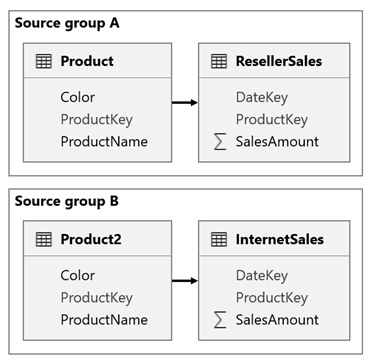
In the report, you add a slicer that filters the page by using the Color column of the Product table. By default, the slicer filters the ResellerSales table, but not the InternetSales table. You then add a hidden slicer by using the Color column of the Product2 table. By setting an identical group name (found in the sync slicers Advanced options), filters applied to the visible slicer automatically propagate to the hidden slicer.
Note
While using sync slicers can avoid the need to create a cross source group relationship, it increases the complexity of the model design. Be sure to educate other users on why you designed the model with duplicate dimension tables. Avoid confusion by hiding dimension tables that you don't want other users to use. You can also add description text to the hidden tables to document their purpose.
For more information, see Sync separate slicers.
Here's some other guidance to help you design and maintain composite models.
For more information related to this article, check out the following resources.
Events
Power BI DataViz World Championships
14 Feb, 16 - 31 Mar, 16
With 4 chances to enter, you could win a conference package and make it to the LIVE Grand Finale in Las Vegas
Learn moreTraining
Learning path
Use advance techniques in canvas apps to perform custom updates and optimization - Training
Use advance techniques in canvas apps to perform custom updates and optimization
Certification
Microsoft Certified: Power BI Data Analyst Associate - Certifications
Erfahren Sie mehr über die Methoden und Best Practices, die den geschäftlichen und technischen Anforderungen für die Modellierung, Visualisierung und Analyse von Daten mit Microsoft Power BI entsprechen.