Note
Access to this page requires authorization. You can try signing in or changing directories.
Access to this page requires authorization. You can try changing directories.
Applies to:  SQL Server 2019 and later Analysis Services
Azure Analysis Services
Fabric/Power BI Premium
SQL Server 2019 and later Analysis Services
Azure Analysis Services
Fabric/Power BI Premium
Calculation groups can significantly reduce the number of redundant measures by grouping common measure expressions as calculation items. Calculation groups are supported in tabular models at the 1500 and higher compatibility level.
Benefits
Calculation groups address an issue in complex models where there can be a proliferation of redundant measures using the same calculations - most common with time intelligence calculations. For example, a sales analyst wants to view sales totals and orders by month-to-date (MTD), quarter-to-date (QTD), year-to-date (YTD), orders year-to-date for the previous year (PY), and so on. The data modeler has to create separate measures for each calculation, which can lead to dozens of measures. For the user, this can mean having to sort through just as many measures, and apply them individually to their report.
Let's first look at how calculation groups appear to users in a reporting tool like Power BI. We'll then look at what makes up a calculation group, and how they're created in a model.
Calculation groups are shown in reporting clients as a table with a single column. The column isn't like a typical column or dimension, instead it represents one or more reusable calculations, or calculation items that can be applied to any measure already added to the Values filter for a visualization.
In the following animation, a user is analyzing sales data for years 2012 and 2013. Before applying a calculation group, the common base measure Sales calculates a sum of total sales for each month. The user then wants to apply time intelligence calculations to get sales totals for month to date, quarter to date, year to date, and so on. Without calculation groups, the user would have to select individual time intelligence measures.
With a calculation group, in this example named Time Intelligence, when the user drags the Time Calculation item to the Columns filter area, each calculation item appears as a separate column. Values for each row are calculated from the base measure, Sales.
Calculation groups work with explicit DAX measures. In this example, Sales is an explicit measure already created in the model. Calculation groups don't work with implicit DAX measures. For example, in Power BI implicit measures are created when a user drags columns onto visuals to view aggregated values, without creating an explicit measure. At this time, Power BI generates DAX for implicit measures written as inline DAX calculations - meaning implicit measures can't work with calculation groups. A new model property visible in the Tabular Object Model (TOM) has been introduced, DiscourageImplicitMeasures. Currently, in order to create calculation groups this property must be set to true. When set to true, Power BI Desktop in Live Connect mode disables creation of implicit measures.
Calculation groups also support Multidimensional Data Expressions (MDX) queries. This means, Microsoft Excel users, which query tabular data models by using MDX, can take full advantage of calculation groups in worksheet PivotTables and charts.
How they work
Now that you've seen how calculation groups benefit users, let's look at how the Time Intelligence calculation group example shown is created.
Before we go into the details, let's introduce some new DAX functions specifically for calculation groups:
SELECTEDMEASURE - Used by expressions for calculation items to reference the measure that is currently in context. In this example, the Sales measure.
SELECTEDMEASURENAME - Used by expressions for calculation items to determine the measure that is in context by name.
ISSELECTEDMEASURE - Used by expressions for calculation items to determine the measure that is in context is specified in a list of measures.
SELECTEDMEASUREFORMATSTRING - Used by expressions for calculation items to retrieve the format string of the measure that is in context.
Time Intelligence example
Table name - Time Intelligence
Column name - Time Calculation
Precedence - 20
Time Intelligence calculation items
Current
SELECTEDMEASURE()
MTD
CALCULATE(SELECTEDMEASURE(), DATESMTD(DimDate[Date]))
QTD
CALCULATE(SELECTEDMEASURE(), DATESQTD(DimDate[Date]))
YTD
CALCULATE(SELECTEDMEASURE(), DATESYTD(DimDate[Date]))
PY
CALCULATE(SELECTEDMEASURE(), SAMEPERIODLASTYEAR(DimDate[Date]))
PY MTD
CALCULATE(
    SELECTEDMEASURE(),
    SAMEPERIODLASTYEAR(DimDate[Date]),
    'Time Intelligence'[Time Calculation] = "MTD"
)
PY QTD
CALCULATE(
    SELECTEDMEASURE(),
    SAMEPERIODLASTYEAR(DimDate[Date]),
    'Time Intelligence'[Time Calculation] = "QTD"
)
PY YTD
CALCULATE(
    SELECTEDMEASURE(),
    SAMEPERIODLASTYEAR(DimDate[Date]),
    'Time Intelligence'[Time Calculation] = "YTD"
)
YOY
SELECTEDMEASURE() -
CALCULATE(
    SELECTEDMEASURE(),
    'Time Intelligence'[Time Calculation] = "PY"
)
YOY%
DIVIDE(
    CALCULATE(
        SELECTEDMEASURE(),
        'Time Intelligence'[Time Calculation]="YOY"
    ),
    CALCULATE(
        SELECTEDMEASURE(),
        'Time Intelligence'[Time Calculation]="PY"
    )
)
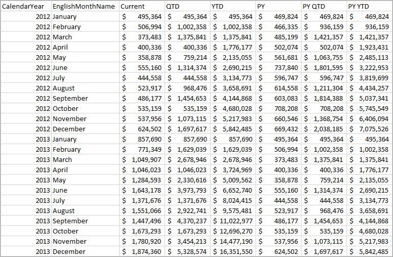
To test this calculation group, execute the following DAX query. Note: MTD, YOY and YOY% are omitted from this query example.
Time Intelligence query
EVALUATE
CALCULATETABLE (
    SUMMARIZECOLUMNS (
        DimDate[CalendarYear],
        DimDate[EnglishMonthName],
        "Current", CALCULATE ( [Sales], 'Time Intelligence'[Time Calculation] = "Current" ),
        "QTD",     CALCULATE ( [Sales], 'Time Intelligence'[Time Calculation] = "QTD" ),
        "YTD",     CALCULATE ( [Sales], 'Time Intelligence'[Time Calculation] = "YTD" ),
        "PY",      CALCULATE ( [Sales], 'Time Intelligence'[Time Calculation] = "PY" ),
        "PY QTD",  CALCULATE ( [Sales], 'Time Intelligence'[Time Calculation] = "PY QTD" ),
        "PY YTD",  CALCULATE ( [Sales], 'Time Intelligence'[Time Calculation] = "PY YTD" )
    ),
    DimDate[CalendarYear] IN { 2012, 2013 }
)
Time Intelligence query return
The return table shows calculations for each calculation item applied. For example, see QTD for March 2012 is the sum of January, February and March 2012.
Dynamic format strings
Dynamic format strings with calculation groups allow conditional application of format strings to measures without forcing them to return strings.
Tabular models support dynamic formatting of measures by using DAX's FORMAT function. However, the FORMAT function has the disadvantage of returning a string, forcing measures that would otherwise be numeric to also be returned as a string. This can have some limitations, such as not working with most Power BI visuals depending on numeric values, like charts.
In Power BI, Dynamic format strings for measures also allow conditional application of format strings to a specific measure without forcing them to return a string and without the use of calculation groups. To learn more, see Dynamic format strings for measures.
Dynamic format strings for time intelligence
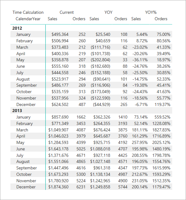
If we look at the Time Intelligence example shown above, all the calculation items except YOY% should use the format of the current measure in context. For example, YTD calculated on the Sales base measure should be currency. If this were a calculation group for something like an Orders base measure, the format would be numeric. YOY%, however, should be a percentage regardless of the format of the base measure.
For YOY%, we can override the format string by setting the format string expression property to 0.00%;-0.00%;0.00%. To learn more about format string expression properties, see MDX Cell Properties - FORMAT STRING Contents.
In this matrix visual in Power BI, you see Sales Current/YOY and Orders Current/YOY retain their respective base measure format strings. Sales YOY% and Orders YOY%, however, overrides the format string to use percentage format.
Dynamic format strings for currency conversion
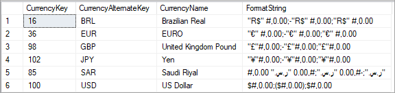
Dynamic format strings provide easy currency conversion. Consider the following Adventure Works data model. It's modeled for one-to-many currency conversion as defined by Conversion types.
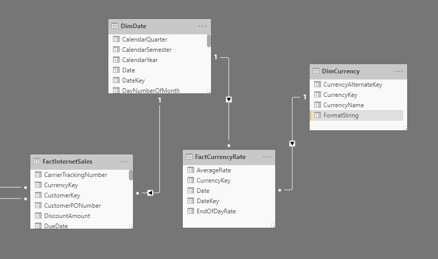
A FormatString column is added to the DimCurrency table and populated with format strings for the respective currencies.
For this example, the following calculation group is then defined as:
Currency Conversion example
Table name - Currency Conversion
Column name - Conversion Calculation
Precedence - 5
Calculation items for Currency Conversion
No Conversion
SELECTEDMEASURE()
Converted Currency
IF(
    //Check one currency in context & not US Dollar, which is the pivot currency:
    SELECTEDVALUE( DimCurrency[CurrencyName], "US Dollar" ) = "US Dollar",
    SELECTEDMEASURE(),
    SUMX(
        VALUES(DimDate[Date]),
        CALCULATE( DIVIDE( SELECTEDMEASURE(), MAX(FactCurrencyRate[EndOfDayRate]) ) )
    )
)
Format string expression
SELECTEDVALUE(
    DimCurrency[FormatString],
    SELECTEDMEASUREFORMATSTRING()
)
Note
Selection expressions for calculation groups can be used to implement automatic currency conversion on calculation groups, removing the need to have two seperate calculation items.
The format string expression must return a scalar string. It uses the new SELECTEDMEASUREFORMATSTRING function to revert to the base measure format string if there are multiple currencies in filter context.
The following animation shows the dynamic format currency conversion of the Sales measure in a report.

Selection expressions
Selection expressions are optional properties defined for a calculation group. There are two types of selection expressions:
- multipleOrEmptySelectionExpression. This selection expression is applied when:
- multiple calculation items have been selected,
- a non-existing calculation item has been selected, or
- a conflicting selection has been made.
- noSelectionExpression. This selection expression is applied when the calculation group is not filtered.
Both of these selection expressions also have a formatStringDefinition dynamic format string expression.
In summary, on a calculation group the following can be defined, for example using TMDL:
...
table Scenarios
	calculationGroup
		...
    multipleOrEmptySelectionExpression = <expression>
        formatStringDefinition = <format string>
    noSelectionExpression= <expression>
        formatStringDefinition = <format string>
...
Note
These expressions, if specified, are only applied for the specific situations mentioned. Selections for a single calculation item are not impacted by these expressions.
Here is an overview of these expressions and their default behavior if not specified:
| Type of selection | Selection expression not defined (default) | Selection expression defined |
|---|---|---|
| Single selection | Selection is applied | Selection is applied |
| Multiple selection | Calculation group is not filtered | Return result of evaluating multipleOrEmptySelectionExpression |
| Empty selection | Calculation group is not filtered | Return result of evaluating multipleOrEmptySelectionExpression |
| No selection | Calculation group is not filtered | Return result of evaluating noSelectionExpression |
Note
Use the model's selectionExpressionBehavior setting to further influence what a calculation group returns when selection expressions are not defined.
SelectionExpressionBehavior model setting
Models have a selectionExpressionBehavior setting that enables further control over how calculation groups in that model behave. This setting accepts the following three values:
- Automatic. This is the default value and is the same as nonvisual. This ensures that your existing models do not change behavior. Models above a future compatibility level set to automatic will use visual instead. There will be an announcement at that time.
- Nonvisual. If the calculation group does not define a multipleOrEmptySelection expression the calculation group returns
SELECTEDMEASURE()and when grouping by the calculation group, subtotal values are hidden. - Visual. If the calculation group does not define a multipleOrEmptySelection expression the calculation group returns
BLANK(). When grouping by the calculation group, subtotal values are determined by evaluating the selected measure in the context of the calculation group.
Use TMDL to set the property on your model:
createOrReplace
    model Model
        ...
        selectionExpressionBehavior: <automatic|nonvisual|visual>
...
Multiple or Empty selection
If multiple selections on the same calculation group are made, the calculation group will evaluate and return the result of the multipleOrEmptySelectionExpression if defined. If this expression has not been defined the calculation group will return the following result if the model's selectionExpressionBehavior setting is set to automatic or nonvisual:
SELECTEDMEASURE()
If the model's selectionExpressionBehavior setting is set to visual, then the calculation group will return:
BLANK()
As an example, let's look at a calculation group called MyCalcGroup that has a multipleOrEmptySelectionExpression configured as follows:
IF (
ISFILTERED ( 'MyCalcGroup' ),
    "Filters: "
         & CONCATENATEX (
  	            FILTERS ( 'MyCalcGroup'[Name] ),
            'MyCalcGroup'[Name],
            ", "
     	   )
)
Now, imagine the following selection on the calculation group:
EVALUATE
{
    CALCULATE (
        [MyMeasure],
        'MyCalcGroup'[Name] = "item1" || 'MyCalcGroup'[Name] = "item2"
    )
}
Here, we select two items on the calculation group, "item1" and "item2". This is a multiple selection and hence the multipleOrEmptySelectionExpression is evaluated and returns the following result: "Filters: item1, item2".
Next, take the following selection on the calculation group:
EVALUATE
{
    CALCULATE (
        [MyMeasure],
        'MyCalcGroup'[Name] = "item4" -- item4 does not exists
    )
}
This is an example of an empty selection, as "item4" does not exist on this calculation group. Therefore, the multipleOrEmptySelectionExpression is evaluated and returns the following result: "Filters: ".
No selection
The noSelectionExpression on a calculation group will be applied if the calculation group has not been filtered. This is mostly used to perform default actions without the need for the user to take action while still providing flexibliity to the user to override the default action. For example, let's look at automatic currency conversion with US Dollar as the central pivot currency.
We can set up a calculation group with the following noSelectionExpression:
IF (
    //Check one currency in context & not US Dollar, which is the pivot currency:
    SELECTEDVALUE (
        DimCurrency[CurrencyName],
        "US Dollar"
    ) = "US Dollar",
    SELECTEDMEASURE (),
    SUMX (
        VALUES ( DimDate[DateKey] ),
        CALCULATE (
            DIVIDE ( SELECTEDMEASURE (), MAX ( FactCurrencyRate[EndOfDayRate] ) )
        )
    )
)
We will also set a formatStringDefinition for this expression:
SELECTEDVALUE(
  DimCurrency[FormatString],
  SELECTEDMEASUREFORMATSTRING()
)
Now, if no currency is selected all currencies will be automatically converted to the pivot currency (US Dollar) as necessary. On top of that, you can still pick another currency to convert to that currency without having to switch calculation items as you would have to do without the noSelectionExpression.
Precedence
Precedence is a property defined for a calculation group. It specifies the order the calculation groups are combined with the underlying measure when using SELECTEDMEASURE() in the calculation item.
Precedence example
Let's look at a simple example. This model has a measure with a specified value of 10, and two calculation groups, each with a single calculation item. We’re going to apply both calculation group’s calculation items to the measure. This is how we set it up:
'Measure group'[Measure] = 10
The first calculation group is 'Calc Group 1 (Precedence 100)' and the calculation item is 'Calc item (Plus 2)':
'Calc Group 1 (Precedence 100)'[Calc item (Plus 2)] = SELECTEDMEASURE() + 2
The second calculation group is 'Calc Group 2 (Precedence 200)' and the calculation item is 'Calc item (Times 2)':
'Calc Group 2 (Precedence 200)'[Calc item (Times 2)] = SELECTEDMEASURE() * 2
You can see calculation group 1 has a precedence value of 100, and calculation group 2 has a precedence value of 200.
By using SQL Server Management Studio (SSMS) or an external tool with XMLA read-write features, like the open-source Tabular Editor, you can use XMLA scripts to create calculation groups and set the precedence values. Here we add "Calc group 1 (Precedence 100)":
{
  "createOrReplace": {
    "object": {
      "database": "CHANGE TO YOUR DATASET NAME",
      "table": "Calc group 1 (Precedence 100)"
    },
    "table": {
      "name": "Calc group 1 (Precedence 100)",
      "calculationGroup": {
        "precedence": 100,
        "calculationItems": [
          {
            "name": "Calc item (Plus 2)",
            "expression": "SELECTEDMEASURE() + 2",
          }
        ]
      },
      "columns": [
        {
          "name": "Calc group 1 (Precedence 100)",
          "dataType": "string",
          "sourceColumn": "Name",
          "sortByColumn": "Ordinal",
          "summarizeBy": "none",
          "annotations": [
            {
              "name": "SummarizationSetBy",
              "value": "Automatic"
            }
          ]
        },
        {
          "name": "Ordinal",
          "dataType": "int64",
          "isHidden": true,
          "sourceColumn": "Ordinal",
          "summarizeBy": "sum",
          "annotations": [
            {
              "name": "SummarizationSetBy",
              "value": "Automatic"
            }
          ]
        }
      ],
      "partitions": [
        {
          "name": "Partition",
          "mode": "import",
          "source": {
            "type": "calculationGroup"
          }
        }
      ]
    }
  }
}
And this script adds "Calc group 2 (Precedence 200)":
{
  "createOrReplace": {
    "object": {
      "database": "CHANGE TO YOUR DATASET NAME",
      "table": "Calc group 2 (Precedence 200)"
    },
    "table": {
      "name": "Calc group 2 (Precedence 200)",
      "calculationGroup": {
        "precedence": 200,
        "calculationItems": [
          {
            "name": "Calc item (Times 2)",
            "expression": "SELECTEDMEASURE() * 2"
          }
        ]
      },
      "columns": [
        {
          "name": "Calc group 2 (Precedence 200)",
          "dataType": "string",
          "sourceColumn": "Name",
          "sortByColumn": "Ordinal",
          "summarizeBy": "none",
          "annotations": [
            {
              "name": "SummarizationSetBy",
              "value": "Automatic"
            }
          ]
        },
        {
          "name": "Ordinal",
          "dataType": "int64",
          "isHidden": true,
          "sourceColumn": "Ordinal",
          "summarizeBy": "sum",
          "annotations": [
            {
              "name": "SummarizationSetBy",
              "value": "Automatic"
            }
          ]
        }
      ],
      "partitions": [
        {
          "name": "Partition",
          "mode": "import",
          "source": {
            "type": "calculationGroup"
          }
        }
      ]
    }
  }
}
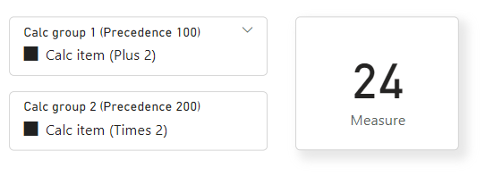
In Power BI Desktop, we have a card visual showing the measure and a slicer for each of the calculation groups in the report view:

When both slicers are selected, we need to combine the DAX expressions. To do that, we start with the highest precedence calculation item, 200, and then replace the SELECTEDMEASURE() argument with the next highest, 100.
So, our highest precedence calculation item DAX expression is:
SELECTEDMEASURE() * 2
And our second highest precedence calculation item DAX expression is:
SELECTEDMEASURE() + 2
Now they're combined by replacing the SELECTEDMEASURE() portion of the highest precedence calculation item with the next highest precedence calculation item, like this:
( SELECTEDMEASURE() + 2 ) * 2
Then if there are more calculation items we continue until we get to the underlying measure. There are only two calculation groups in this model, so we now replace the SELECTEDMEASURE() with the measure itself, like this:
( ( [Measure] ) + 2 ) * 2
As our Measure = 10, this is the same as:
( ( 10 ) + 2 ) * 2
When there are no more SELECTEDMEASURE() arguments, the combined DAX expression is evaluated:
( ( 10 ) + 2 ) * 2 = 24
In Power BI Desktop, when both calculation groups are applied with a slicer, the measure output looks like this:
But keep in mind, the combination is nested in such a way that the output won't be 10 + 2 * 2 = 14 as you see here:
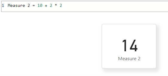
For simple transformations, the evaluation is from lower to higher precedence. For example, 10 has 2 added, then it's multiplied by 2. In DAX, there are functions like CALCULATE that apply filters or context changes to inner expressions. In this case, the higher precedence alters a lower precedence expression.
Precedence also determines which dynamic format string is applied to the combined DAX expression for each measure. The highest precedence calculation group dynamic format string is the only one applied. If a measure itself has a dynamic format string, it's considered a lower precedence to any calculation group in the model.
Precedence with averages example
Let's look at another example using same model as shown in the time intelligence example described earlier in this article. But this time, let's also add an Averages calculation group. The Averages calculation group contains average calculations that are independent of traditional time intelligence in that they don't change the date filter context - they just apply average calculations within it.
In this example, a daily average calculation is defined. Calculations such as average barrels of oil per day are common in oil-and-gas applications. Other common business examples include store sales average in retail.
While such calculations are calculated independently of time intelligence calculations, there may well be a requirement to combine them. For example, a user might want to see barrels of oil per day YTD to view the daily oil rate from the beginning of the year to the current date. In this scenario, precedence should be set for calculation items.
Our assumptions are:
Table name is Averages.
Column name is Average Calculation.
Precedence is 10.
Calculation items for Averages
No Average
SELECTEDMEASURE()
Daily Average
DIVIDE(SELECTEDMEASURE(), COUNTROWS(DimDate))
Here's an example of a DAX query and return table:
Averages query
EVALUATE
    CALCULATETABLE (
        SUMMARIZECOLUMNS (
        DimDate[CalendarYear],
        DimDate[EnglishMonthName],
        "Sales", CALCULATE (
            [Sales],
            'Time Intelligence'[Time Calculation] = "Current",
            'Averages'[Average Calculation] = "No Average"
        ),
        "YTD", CALCULATE (
            [Sales],
            'Time Intelligence'[Time Calculation] = "YTD",
            'Averages'[Average Calculation] = "No Average"
        ),
        "Daily Average", CALCULATE (
            [Sales],
            'Time Intelligence'[Time Calculation] = "Current",
            'Averages'[Average Calculation] = "Daily Average"
        ),
        "YTD Daily Average", CALCULATE (
            [Sales],
            'Time Intelligence'[Time Calculation] = "YTD",
            'Averages'[Average Calculation] = "Daily Average"
        )
    ),
    DimDate[CalendarYear] = 2012
)
Averages query return
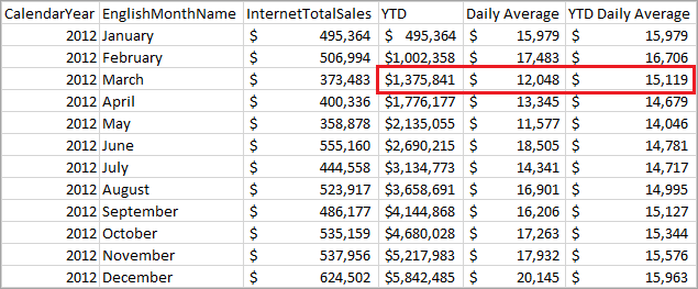
The following table shows how the March 2012 values are calculated.
| Column name | Calculation |
|---|---|
| YTD | Sum of Sales for Jan, Feb, Mar 2012 = 495,364 + 506,994 + 373,483 |
| Daily Average | Sales for Mar 2012 divided by # of days in March = 373,483 / 31 |
| YTD Daily Average | YTD for Mar 2012 divided by # of days in Jan, Feb, and Mar = 1,375,841 / (31 + 29 + 31) |
Here's the definition of the YTD calculation item, applied with precedence of 20.
CALCULATE(SELECTEDMEASURE(), DATESYTD(DimDate[Date]))
Here's Daily Average, applied with a precedence of 10.
DIVIDE(SELECTEDMEASURE(), COUNTROWS(DimDate))
Since the precedence of the Time Intelligence calculation group is higher than that of the Averages calculation group, it's applied as broadly as possible. The YTD Daily Average calculation applies YTD to both the numerator and the denominator (count of days) of the daily average calculation.
This is equivalent to the following expression:
CALCULATE(DIVIDE(SELECTEDMEASURE(), COUNTROWS(DimDate)), DATESYTD(DimDate[Date]))
Not this expression:
DIVIDE(CALCULATE(SELECTEDMEASURE(), DATESYTD(DimDate[Date])), COUNTROWS(DimDate)))
Sideways recursion
In the Time Intelligence example above, some of the calculation items refer to others in the same calculation group. This is called sideways recursion. For example, YOY% references both YOY and PY.
DIVIDE(
    CALCULATE(
        SELECTEDMEASURE(),
        'Time Intelligence'[Time Calculation]="YOY"
    ),
    CALCULATE(
        SELECTEDMEASURE(),
        'Time Intelligence'[Time Calculation]="PY"
    )
)
In this case, both expressions are evaluated separately because they are using different calculate statements. Other types of recursion aren't supported.
Single calculation item in filter context
In our Time Intelligence example, the PY YTD calculation item has a single calculate expression:
CALCULATE(
    SELECTEDMEASURE(),
    SAMEPERIODLASTYEAR(DimDate[Date]),
    'Time Intelligence'[Time Calculation] = "YTD"
)
The YTD argument to the CALCULATE() function overrides the filter context to reuse the logic already defined in the YTD calculation item. It's not possible to apply both PY and YTD in a single evaluation. Calculation groups are only applied if a single calculation item from the calculation group is in filter context.
Ordering
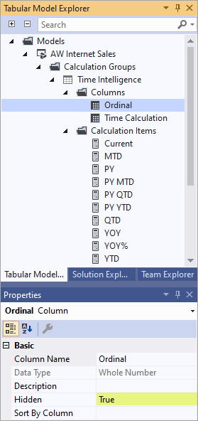
By default, when a column from a calculation group is placed in a report, calculation items are ordered alphabetically by name. The order in which calculation items appear in a report can be changed by specifying the Ordinal property. Specifying calculation item order with the Ordinal property doesn't change precedence, the order in which calculation items are evaluated. It also doesn't change the order in which calculation items appear in Tabular Model Explorer.
To specify the ordinal property for calculation items, you must add a second column to the calculation group. Unlike the default column where Data Type is Text, a second column used for ordering calculation items has a Whole Number data type. The only purpose for this column is to specify the numeric order in which calculation items in the calculation group appear. Because this column provides no value in a report, it's best to set the Hidden property to True.
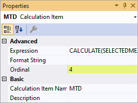
After a second column is added to the calculation group, you can specify the Ordinal property value for calculation items you want to order.
To learn more, see To order calculation items.
Create a calculation group
Calculation groups are supported in Visual Studio with Analysis Services Projects VSIX update 2.9.2 and later. Calculation groups can also be created by using Tabular Model Scripting Language (TMSL) or the open source Tabular Editor.
To create a calculation group by using Visual Studio
In Tabular Model Explorer, right-click Calculation Groups, and then click New Calculation Group. By default, a new calculation group has a single column and a single calculation item.
Use Properties to change the name and enter a description for the calculation group, column, and default calculation item.
To enter a DAX formula expression for the default calculation item, right-click and then click Edit Formula to open DAX Editor. Enter a valid expression.
To add more calculation items, right-click Calculation Items, and then click New Calculation Item.
To order calculation items
In Tabular Model Explorer, right-click a calculation group, and then click Add column.
Name the column Ordinal (or something similar), enter a description, and then set the Hidden property to True.
For each calculation item you want to order, set the Ordinal property to a positive number. Each number is sequential, for example, a calculation item with an Ordinal property of 1 appears first, a property of 2 appears second, and so on. Calculation items with the default -1 aren't included in the ordering, but appear before ordered items in a report.
Considerations
As soon as a calculation group is added to a semantic model, Power BI reports will use the variant data type for all measures. If afterwards, all calculation groups are removed from the model the measures will be returned to their original data types again.
Limitations
Object level security (OLS) defined on calculation group tables isn't supported. However, OLS can be defined on other tables in the same model. If a calculation item refers to an OLS secured object, a generic error is returned.
Row level security (RLS) isn't supported. Define RLS on tables in the same model, but not on calculation groups themselves (directly or indirectly).
Detail Rows Expressions aren't supported with calculation groups.
Smart narrative visuals in Power BI aren't supported with calculation groups.
Implicit column aggregations in Power BI aren't supported for models with calculation groups. Currently, if DiscourageImplicitMeasures property is set to false (default), aggregation options appear, however they cannot be applied. If DiscourageImplicitMeasures is set to true, aggregation options don't appear.
When creating Power BI reports using LiveConnection, Dynamic format strings aren't applied to report-level measures.