Conditional Formatting - Not working in odd cells where it should be???

Question

Hey,

I have a sheet where I'd applied the same rule to different blocks of numbers in the same column (I can't remember why I did it this way, all I can think is that because I'm not very good with conditional formats I did them all separately).

Now I've tried to use a single rule to cover them all to make it a neater sheet.  However, for some reason the rule isn't working for odd cells where is should / has in the past using the old multiple series of rules.  I can't figure out why.

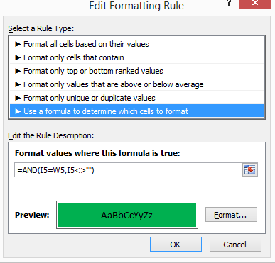
The rule I'm using is: =AND(I5=W5,I5<>"") highlight green, see screenshot.

I've applied a screenshot below of where the error is occurring.  It's also happening in 1 cell above, which is in the middle of cells that are highlighted correctly.

I added the condition by highlighting the entire column W and entering the row number for the first cell that I want the rule to apply to (row 5).

Any ideas what I'm doing wrong?

Cheers.

Answer 1

Hi,

My guess would be that in the rows that aren't getting formatted to values aren't the same as they appear in the cell. Try this for a pair of cells you think should be formatted.

=I20=W20

That has to return TRUE for the cell to be formatted and if it returns FALSE then the values aren't the same. You could try this CF formula.

=AND(ROUND(I5,2)=ROUND(W5,2),I5<>"")

Answer 2

That link didn't work for me, try this one:

https://onedrive.live.com/redir?resid=8112052B896CBD6!165&authkey=!AGnLhAhyTWigx80&ithint=file%2c.xlsx

Answer 3

Did you try my suggestion?

Just select entire column and give formula as 

=AND(I1=W1,I1<>"")

Or in case you want to do round then,

=AND(ROUND(I1,2)=ROUND(W1,2),I1<>"")

it will work, I just tried on your linked file.

Answer 4

That link didn't work for me, try this one:

https://onedrive.live.com/redir?resid=8112052B896CBD6!165&authkey=!AGnLhAhyTWigx80&ithint=file%2c.xlsx

Hi,

I corrected the conditional formatting and saved a working version to my Onedrive. It's called Hours Log.xlsx

Link

Answer 5

https://onedrive.live.com/redir?resid=D62CBB3CF367F163%21166

In this sheet (squares tab), I have divided up the UK into OS gridsquares.  Basically, a small square should turn yellow if there is anything in Column D corresponding to that square.

Column B has all the squares.  Column D has callsigns contacted in those squares.  The "map" over to the right is arranged in squares.  I have set up conditional formatting to turn the cell background yellow if there is anything in column D.

This works all the way through the map - except for large square J (Northern Ireland).  This is cells B139 to B193 in the lookup vector, and cells T79 to AC88 on the map display and where the conditional formatting SHOULD take effect.

I just can't fathom this one out.  I know SOME conditional formatting is working in those cells because the background has turned turquoise if the cell is empty (that's the first condition).  I've checked using formulas that the logic is seeing the cells as equal value (and it is), and that cell formats are the same etc.

Can anyone solve this one?

Tom