MS Excel INDEX, MATCH combined with COUNTIF

Question

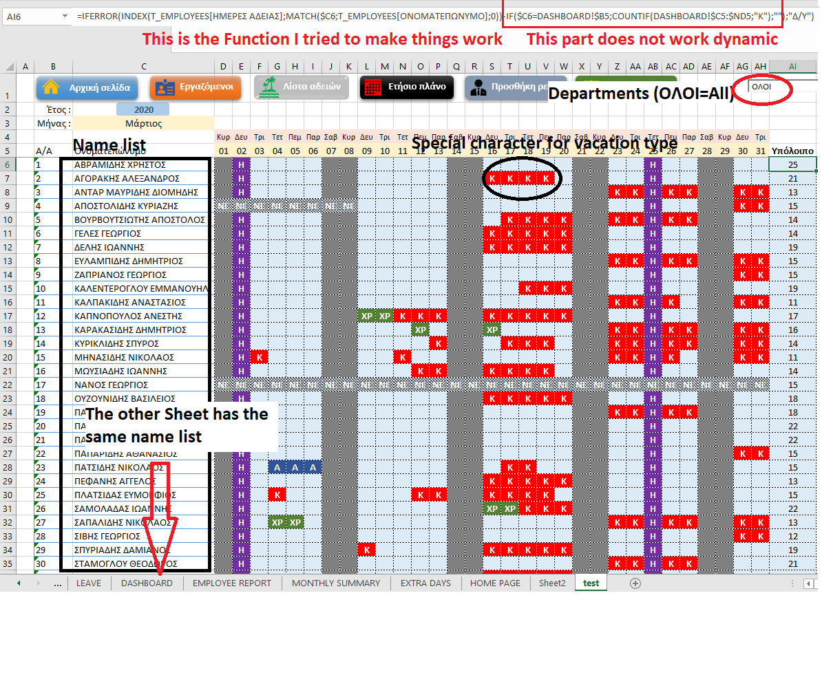
Hello, I am trying to calculate data from another sheet based on some criteria. I want to search and match the name of the first list with a second one in another sheet, then from the second list (which is Table)

I have 2 sheets, first one has the annual Dashboard of all employees (365 days) and there are symbols that separates type of leave, for example U is unpaid or S is sick etc, the second is a table, with employees names at the first column and in the rest columns are vacation types, (Column2 = Unpaid, Column3 = Sick etc) and I want to count per employee and per vacation type their leaves. Finaly I want on the second sheet to contain my company's employees name and the totals of every vacation type.

So, I tried using INDEX and MATCH to find employee and with a simple IF function (cause the 2 tables are identically) was easy to bring the final count.

But, after this video ( https://www.youtube.com/watch?v=fDB1Ktyhp3Y ) I tried to make a Drop down list with our company's Departments and when I select the department filters the first column and shows me only selected department's employees, but, the count function did never work.

I will appreciate your help on this. Thank you very much.

Here is a picture of my project, it is in Greek but I added some comments to help.

Answer 1

Everything can be dynamic - height, width, the offsets. You can also use INDEX - which has an odd usage, like this, with that hanging comma at the end to use all the columns of the range:

=COUNTIF(INDEX(DASHBOARD!$B$5:$$ZZ$1000,MATCH(C6,DASHBOARD!$B$5:$B$10000,FALSE),),"K")

And if you are afraid of row insertions between 4 and 5, you can offset from B5 and subtract 1 from the MATCH return....

Answer 2

I would use a formula like this, with names starting in cell B5 of DASHBOARD:

=COUNTIF(OFFSET(DASHBOARD!$B$4,MATCH(C6,DASHBOARD!$B$5:$B$10000,FALSE),0,1,366),"K")

Answer 3

The weird thing with comma at the end of INDEX we use to say the formula, look all the columns in the given range? Otherwise, it returns #REF. If I delete comma what does it search?

So, in sheet DASHBOARD my range is a Table called T_DASHBOARD and I turn yours formula to this : COUNTIF(INDEX(T_DASHBOARD;MATCH(C6;T_DASHBOARD[[#All];[Column367]];FALSE););"Κ").

It works!

Thank you!

Answer 4

Great! It's always nice to have multiple options...