Conditional Formatting Question - Excel (AND,ISNUMBER,LARGE)

Question

Hi, 

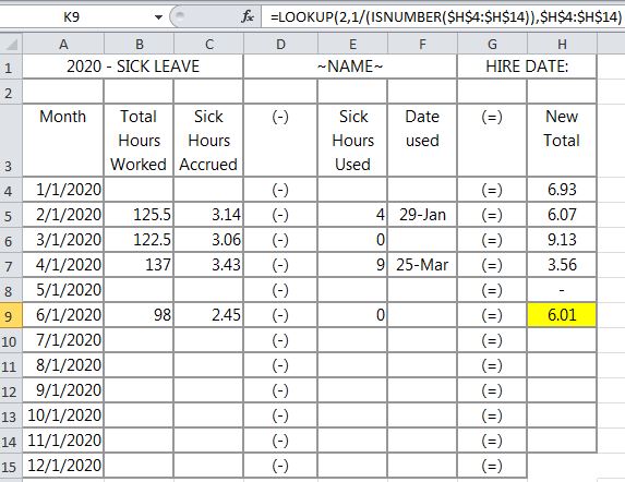
I can't write this correctly.  I'd like to highlight the cells in the H column that are a number (ISNUMBER) while matching them with the greatest date (LARGE) in the column A. 

I tried: 

=AND(ISNUMBER($H4),$A4=LARGE($A$4:$A$15,1))

H4 contains 6.93

A4 contains 1/1/2020 - correctly formatted as date 

Conditional formula: =$A4=LARGE($A$4:$A$15,1) works fine, standalone.  The value 12/1/2020 highlights.  

Conditional formula: =ISNUMBER($H4) highlights the correct values, standalone. 

I really need this formula to highlight H9 as it reflects the LARGE date 06/01 and the ISNUMBER cell H9 that has the value 6.01 and the largest date with a number in column H. 

I don't know where I'm going wrong.  My syntax is bad.  I'd appreciate any support I'm given. Thank you.

2020 - SICK LEAVE	~NAME~	HIRE DATE:
Month	Total Hours Worked	Sick Hours Accrued	(-)	Sick Hours Used	Date used	(=)	New Total
1/1/2020			(-)			(=)	6.93
2/1/2020	125.5	3.14	(-)	4	29-Jan	(=)	6.07
3/1/2020	122.5	3.06	(-)	0		(=)	9.13
4/1/2020	137	3.43	(-)	9	25-Mar	(=)	3.56
5/1/2020			(-)			(=)	-
6/1/2020	98	2.45	(-)	0		(=)	6.01
7/1/2020			(-)			(=)
8/1/2020			(-)			(=)
9/1/2020			(-)			(=)
10/1/2020			(-)			(=)
11/1/2020			(-)			(=)
12/1/2020			(-)			(=)

Answer 1

Hello,

Looks like you want to find the last numeric value in column H. You don't need additional criteria to check against Date column, as finding the last numeric value will do the job.

To find the value of the last non-empty cell in a row or column, you can use the LOOKUP() function. This formula is not an array formula and has performance advantages.

If you want to find the last numeric value in column H use this formula:

=LOOKUP(2,1/(ISNUMBER($H$4:$H$14)),$H$4:$H$14)

To highlight it, enter the following conditional Formatting:

=H4=LOOKUP(2,1/(ISNUMBER($H$4:$H$14)),$H$4:$H$14)

Let me know if you find this helpful!

Answer 2

Try a CFR on H4:H99 based on the following formula.

=AND(ISNUMBER($H4), $A4=AGGREGATE(14,7,  ($A$4:$A$99)/($H$4:$H$99<>""), 1))

Later versions of Excel could use MAXIFS to find the largest date where column H is not blank. Earlier versions could use INDEX in the method described in MINIF, MAXIF and MODEIF.

Answer 3

Hi Robin,

I will be happy to help you understand the logic behind the above Lookup() function usage.

The LOOKUP function assumes data is sorted,and works based on approximate match. More precisely, a Lookup formula searches for exact match first. If the lookup value is greater than all values in the lookup array, default behavior is to "fall back" to the previous value.

=LOOKUP(2,1/(ISNUMBER($H$4:$H$14)),$H$4:$H$14)

This formula exploits this behavior by creating an array that contains only 1s and errors, then deliberately looking for the value 2, which will never be found.

Because the highest value you can get in your second part of the formula is 1/1=1

You can use any big number that is greater than numbers in your lookup vector, for instance,

=LOOKUP(100000,$H$4:$H$14) This will also results in the last numeric value, because it won't able to find 100000 and "fall back" to the last value.

To read more about the concept of intentionally looking for a value that won't ever appear, read about Big Numbers.

Source.

Hope this helps!

Answer 4

Hello,

Looks like you want to find the last numeric value in column H. You don't need additional criteria to check against Date column, as finding the last numeric value will do the job.

To find the value of the last non-empty cell in a row or column, you can use the LOOKUP() function. This formula is not an array formula and has performance advantages.

If you want to find the last numeric value in column H use this formula:

=LOOKUP(2,1/(ISNUMBER($H$4:$H$14)),$H$4:$H$14)

To highlight it, enter the following conditional Formatting:

=H4=LOOKUP(2,1/(ISNUMBER($H$4:$H$14)),$H$4:$H$14)

Let me know if you find this helpful!

Bek,

You are amazing!  Thank you so much for your help.  

I had to remove the other formulas I'd listed in the conditional formatting box (prioritizing wasn't helping - stopping "if true"). 

If you can help me one more time: 

1. I have used LOOKUP (H,V) functions in the past to retrieve information but not in this method.  I'm not understanding how to use LOOKUP in this fashion and have only basic experience and can locate information in columns in the result vector to the right.  I am not familiar with using the divide or using an integer in order to get information.  I'll probably have more difficult problems like this to solve and would like to know how you came up with this response. 

I only recently earned an Excel Expert cert and am capable of just basic functions, lookups, etc.  Your answer is so much better!

Thank you so much! You saved my workbook!

Robin

Answer 5

Hi, 

Your reply works as well. You are another amazing Excel champ.

You saved my workbook, as well.  

I won't even ask how this formula works.  

Thank you so much! Your support is very appreciated :)

Robin