Excel Not adding decimals correctly when adding a decimal to a formula

Question

Ok So I created a series of numbers by adding +10.128 to the cell on the row above!

See the error on cell E17 answer should be the same as Cell G17 242682.248000

This error throws out my tests with VBA

I have also seen this with the worksheet function Mod

the answer in cell E39 is wrong

Answer 1

I created a series of numbers by adding +10.128 to the cell on the row above!

See the error on cell E17 answer should be the same as Cell G17 242682.248000

This is a common problem, because most decimal fractions cannot be represented exactly in 64-bit binary floating-point, which is what Excel uses for storing numeric values internally and for performing arithmetic.

Moreover, the binary approximation of a particular decimal fraction might vary depending on the magnitude of the number. That is why, for example, 10.01 - 10 = 0.01 returns FALSE(!). The approximation of 0.01 in 10.01 differs from the approximation of 0.01 itself.

In general, the work-around is: whenever we expect a calculation that involves decimal fractions to be accurate to some number of decimal places, explicitly round to that number of decimal places -- and not to an arbitrary number, as some people suggest.

In your example, change =E15+F16 to =ROUND(E15+F16, 3) .

---

However, we cannot duplicate the misbehavior with just the values that you provided. The value that is displayed in E15 (242661.992) must have been calculated. It, too, should be rounded, as a matter of principle.

You can confirm that E15 is not the exact binary approximation of the displayed value by entering the formula

=SUM(E15, -(E15 & "")), formatted as Scientific.

FYI, we cannot write simply =E15-(E15 & "") because sometimes Excel arbitrarily replaces the infinitesimal difference of the last subtraction in a formula with exactly zero. (sigh)

Answer 2

I'm not sure if there is a still some misunderstanding in your mind. So I'll annotate the VBA step-by-step. Forgive me if this is unnecessary or TMI.

---

Val1 = CDec(Sheet4.Range("D45").Value) ' displays on sheet and VBA locals 3777131679055870 actually 3777131679055872

No, Val1 is __actually__ 3777131679055870, even though D45 is exactly 3777131679055872, and type Decimal is capable of representing the greater precision.

I assume that D45 contains the value that was previously in D39, namely =(C1-1)^2^52, where C1 contains the value returned by =1.83869171142578 + 1.33E-15. IOW, D45 is exactly the integer 3777131679055872, which Excel and VBA display as 3777131679055870.

If you had written CDec("3777131679055872"), Val1 would indeed have the value 3777131679055872 because VBA interprets the entire numeric text. In contrast, Excel interprets only up to the first 15 significant digits (unrounded), replacing any digits to the right with zero.

But for CDec(Range("D45")), VBA first converts Range("D45") to text as it would for display. And like Excel, for type Double, VBA converts only up to the first 15 significant digits (rounded), replacing any digits to the right with zero. So it is effectively CDec("3777131679055870").

In general, if we want a type Decimal value with the full precision of the type Double value, we must write:

Val1 = CDec(Range("D45")) + ( Range("D45") - (Range("D45") & "") )

Note the highlighted parentheses around the subexpression. Arithmetically, they are redundant. But they are needed here in order to ensure that Range("D45") is treated as type Double, not converted to type Decimal left-to-right in the same way that CDec does, thereby losing precision. PS.... Or if you prefer, write CDec(Range("D45") - (Range("D45") & "")).

That is effectively the same calculation that you do for Val3, to wit:

Val2 = WorksheetFunction.Sum(Sheet4.Range("D45").Value, -1 * (Sheet4.Range("D45").Value & "")) '= 2 in VBA locals window
Val3 = Val1 + Val2 ' 3777131679055872 in VBA locals window

---

Ans = Evaluate("MOD(" & Val3 & "," & (2 ^ 32) & ")")
Debug.Print Ans '4294967294 'wrong

"MOD(" & Val3 & "," & 2 ^ 32 & ")" becomes the string "MOD(3777131679055872,4294967296)".

However, when Evaluate passes the string to Excel, Excel interprets 3777131679055872 as 3777131679055870 for the reason mentioned above, to wit: Excel interprets numeric text only up to the first 15 significant digits (unrounded), replacing any digits to the right with zero.

Thus, Excel evaluates "MOD(3777131679055870,4294967296)", despite the increased precision of type Decimal Val3.

The important take-away is: when we use Evaluate, it is Excel, not VBA, that interprets the formula and performs the calculation -- with all of its limitation.

---

Ans = ModBig(Val3, 2 ^ 32)
Debug.Print Ans ' 0 correct

This produces the correct result because the ModBig parameters are type Variant by default.

Thus, since Val3 is type Decimal, "number" in ModBig is subtype Decimal. And in the left-to-right evaluation of the "modulo" expression, all calculations are performed with type Decimal precision.

---

However, it was not necessary to resort to type Decimal in order to get the same result in VBA as we get in Excel (D39 and E39).

To demonstrate, the following type Double arithmetic correctly returns a modulo of zero.

Sub doit()
Dim n As Double, d As Double, m As Double
Range("D45").Formula = "=3777131679055870+2" ' effectively =(C1-1)*2^52
n = Range("D45")
d = 2 ^ 32
m = n - d * Int(n / d)
MsgBox m
End Sub

In fact, it might have been your (mis)use of type Decimal that led to the incorrect results, with or without the use Evaluate("MOD...").

Answer 3

I'm glad you appreciated the details. Not everyone does -- even though they need to hear them in order to understand their problem.

---

I was re-writing all the Modulus calc in VBA and VBA was giving me the 4294967290 answer which was correct, not Zero

FYI, VBA has the same arbitrary display limitations as Excel does, namely: up to 15 significant digits, rounded.

But I do not understand your comment, to wit: VBA gives "the 4294967290 answer which was correct, not Zero".

Although there are instances where the result of VBA arithmetic might differ from Excel arithmetic, this is not one of them.

To demonstrate:

Sub demo()
Dim c1 As Double, d39 As Double, e39 As Double
Dim sC1 As String, sD39 As String
c1 = 1.83869171142578 + 1.33226762955019E-15
d39 = (c1 - 1) * 2 ^ 52
e39 = d39 - 2 ^ 32 * Int(d39 / 2 ^ 32)
sC1 = Replace(" + " & c1 - (c1 & ""), "+ -", "- ")
sD39 = Replace(" + " & d39 - Format(d39, "0"), "+ -", "- ")
MsgBox "C1: " & c1 & sC1 & _
vbNewLine & "D39: " & "(C1-1)*2^52 = " & Format(d39, "0") & sD39 & _
vbNewLine & "E39: MOD(D39,2^32) = " & e39
End Sub

The result is:

C1: 1.83869171142578 + 1.33226762955019E-15

D39: (C1-1)*2^52 = 3777131679055870 + 2
E39: MOD(D39,2^32) = 0

Answer 4

I have also seen this with the worksheet function Mod

the answer in cell E39 is wrong

For these sorts of questions, it is best to upload an example Excel file that demonstrates the problems to a file-sharing website, and post the download URL in a response. I like box.net/files; others like dropbox.com. You might like onedrive.live.com because the login is the same as this forum. But I don't trust "onedrive".

At the very least, you should show us what is in C1, formatted to display 15 significant digits. And based on my previous response, you now know that it would be prudent to also show us the result of =SUM(C1, -(C1 & "")) formatted as Scientific with at least 2 decimal places. Also show us the results of =SUM(D39, -(D39 & "")).

---

Again, you should explicitly round the calculation in D1 to the precision that you expect to be accurate.

Perhaps =ROUND((C1-1)*2^52, 0) .

But I suspect that is not the issue here. Instead, I suspect the issue is: Excel formats only up to the first 15 significant digits, and the value in D39 is actually the exact integer 3777131679055872, an exact multiple of 2^32. So, the MOD expression in E39 is correct to return zero.

Your own experiment in D40 demonstrates that the value in D39 is not what it appears to be. Because if it were, the calculations in E39 and E40 would have the same results.

Instead, let's assume that the MOD calculation in E39 is correct, and the value in D39 is an exact multiple of 2^32. Then:

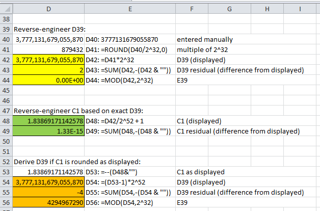
D41 calculates an exact multiple of 2^32 close to the value displayed in D40, namely 879432.

D42 calculates the exact integer that should be in D39, namely 879432 * 2^32.

Contrary to everything you might read, Excel calculations are __not__ limited to 15 significant digits.

Instead, Excel can accurately calculate all integers up to 9,007,199,254,740,992 (2^53), which is 16 digits. Since that is larger than the expected integer in D39, we can expect the calculation in D42 to be an exact integer.

And as the calculation in D43 demonstrates, the value in D42 is really 3,777,131,679,055,872 -- 3777131679055870 displayed in D42 plus 2, the residual displayed in D43.

We cannot see the last digit because, again, Excel arbitrarily formats only the first 15 significant digits (rounded), replacing any digits on the right with zeros.

Based on the correct value in D42, we see in D44 that MOD(D39, 2^32) correctly returns zero.

---

Possible TMI follows....

In D48, we reverse-engineer what your value might be in C1, based on the correct value for D39, which we calculate in D42.

D49 shows the residual difference from what Excel formats in D48. In other words, the value in D48 is actually

1.83869171142578 + 1.33E-15 (approximately).

PS.... In general, because you format E39 as Number with 2 decimal places, we do not really know that it is exactly zero. We can only recognize exact zero by formatting as Scientific (0.00E+00) or by testing =E39=0 (TRUE). Even when formatted as General, 0 might not be exactly zero sometimes. Again, for a dispositive explanation, it is best to provide an example Excel file, not images or descriptions, which are subject to interpretation.

However, in this particular case, because we multiply C1 by such a large factor (2^52), the residual can only be 1.33E-15 (3*2^-51), due to the limited precision of 64-bit BFP. Even 4*2^-51 (1.78E-15) and 2*2^-51 (8.88E-16) would cause visibly different results in E39.

---

The calculations in D53:D56 demonstrate the importance of the residual difference that Excel does not normally display.

In D53, we round D48 to the displayed 15 significant digits.

Then we derive the value in D54 with a formula similar to your formula in D1.

Note that D54 is 3,777,131,679,055,866 -- 3777131679055870 displayed in D54 minus 4, the residual (-4) displayed in D55. It is not 3,777,131,679,055,872, which we presume D39 actually is.

And MOD(D54,2^32) in D56 is 4294967290, not zero as your E39 is.

So, we need the hidden residual difference in C1 in order to calculate D39 and E39 correctly.

Answer 5

Once again thanks for your response and detail.

what I meant by "wrong" is that that line of code gives me a incorrect answer

You have once again explained why the answer is actually correct but different because of how Excel interprets numbers.

Thanks Again.