Need help deciphering LINEST function for Excel.

Question

Hello, so I have some data I am manipulating for a C# project. I am trying to calculate a 6 term polynomial and need to create a moving average and use regression to create this moving average. I was told by a previous worker for the company I work for who does not work here anymore to use

=LINEST(G1:G709,F1:F709^{1,2,3,4,5,6})

It's my understanding that G1:G709 refers to the known x data and F1:F709 refers to the known y data with the exponents referring to the terms (I think). Now I am kind of confused as to what actually is going on here. Like I want to write a function that replicates the LINEST function but idk what is actually going on per say.

If someone could help explain what is going on here that would be great.

Answer 1

It's the other way round: G1:G709 is the range with the y-values and F1:F709 is the range with the x-values.

F1:F709^{1,2,3,4,5,6} represents x, x^2, x^3, x^4, x^5 and x^6.

The result of this LINEST formula will be spread over 7 cells in a row. The first number is the coefficient of x^6, the second one the coefficient of x^5, etc., and the 7th and last number is the constant (intercept).

A simplified example:

The y-values in G1:G6 are the result of =1*F1^6+2*F1^4-8

The numbers in I1:O1 are the coefficients and intercept.

Answer 2

So if I were to use the LINEST function on my data I get this,

.

I went on Desmos.com and wrote out the 6th term polynomial but like I don't understand how the numbers are being outputted. Now for the first of the seven terms in column J how is -1.3379E-14 produced mathematically?

Answer 3

I don't know how Excel computes the result of LINEST - most probably some kind of least squares algorithm.

In your screenshot, the numbers such as -1.3379E-14 are so small that the actual numbers must be 0, and the result returned by Excel is a rounding error. So the result basically says that the data are approximated by a straight line y=-0.54712*x+1136.352

(joeu2004 will probably correct me)

Answer 4

This is an array version of LINEST which allows polynomial regression. The ^{1,2,3,4,5,6} portion is raising each entry in the range F1:F709 to the powers of 1, 2, 3, 4, 5, and 6.

Suppose you have two ranges (G1:G709 and F1:F709 in your case) in mine:

Polynomial Regression:
T	Res
(°K)	(ohm-cm)
300	4.70E+02
320	5.49E+02
340	6.36E+02
360	7.29E+02
380	8.21E+02
400	8.59E+02
420	7.03E+02
440	4.85E+02
460	2.88E+02
480	1.68E+02
500	9.90E+01

The 6 order polynomial regression can be calculated as follows:

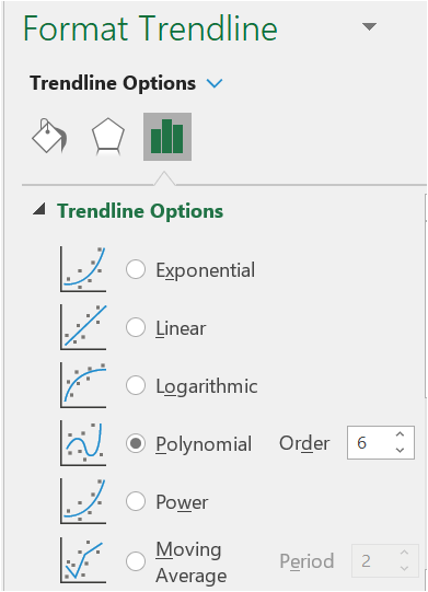
This is identical to what the charting tool does when you add a trend line and choose the option Polynomial, Order 6:

(Note that Moving Average is a separate option)

In my example Res are the known Y-values and T are the known X-values and I am displaying all the stats and suppressing the errors (blank items).

The formula in the purple cell and over the entire rectangle is:

{=IFNA(LINEST(Res,T^{1,2,3,4,5,6},,1),"")}

I have setup the formula to output all the statistics. You can see what each is here: https://support.microsoft.com/en-us/office/linest-function-84d7d0d9-6e50-4101-977a-fa7abf772b6d?ns=excel&version=90&syslcid=1033&uilcid=1033&appver=zxl900&helpid=xlmain11.chm60097&ui=en-us&rs=en-us&ad=us

The numbers in the first two columns above are:

m1	B
se1	seb
r^2^	sey
F	Df
ssreg	ssresid