Automated RAG status formulas using dates

Question

I have an excel spreadsheet where I would like the RAG status to autofill with the appropriate RAG colour appearing in column F. The RAG status would be based on whether a project is on time based on dates.

Column C = Planned completion date

Column D = Forecast/Actual completion date

Column F = RAG status

So for example

F1 would autofill RED if the date in D1 is 30 days later than the date in C1

F1 would autofill AMBER if the date in D1 is less than 30 days later than the date in C1 but more 14 days

F1 would autofill GREEN if the date in D1 is less than 14 days greater than the date in C1

I've tried to use conditional formatting but I can't work out the formula I need to reflect the relationship between the two dates.

Any help would be greatly appreciated!!!

Answer 1

Hi V_R_G_45,

Would you be able to share a link to the file on OneDrive so I can further investigate the issue? Please make sure to remove any personal information before sending. Thanks in advance.

https://support.microsoft.com/en-us/office/shar...

Kind Regards.

Answer 2

Hi Jen,

Here it is. I tried to see if doing the formulas for each row would resolve the problem but it hasn't

Hi,

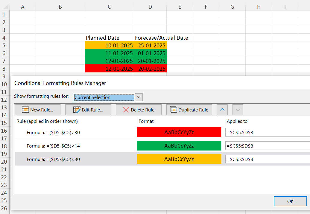
In a cell > MS Excel applies the Conditional Formatting rules > from top-top-bottom.

In the screenshot above:

1st) MS Excel will apply the Red Rule - if it is true.

If the 1st Rule is not true,

2nd) MS Excel will apply the Amber Rule - if it is true.

If the 2nd Rule is not true,

3rd) MS Excel will apply the Green Rule - if it is true.

e.g. In the screenshot above, D6 - C6 = -10

1st) MS Excel will apply the Red Rule - it is not true because -10 IS NOT greater than 30.

2nd) MS Excel will apply the Amber Rule - yes, it is true because -10 IS less than 30.

MS Excel will apply the Amber rule.

SOLUTION

The Conditional Formatting rules should be in the following sequence.

1st - Red Rule

2nd - Green Rule

3rd - Amber Rule

You may move the rules up/down > by clicking on the up-arrow/down-arrow > next to Duplicate Rule option in the Conditional Formatting Rules Manager dialog box.

Please respond if You require further assistance. I will try My best to be of help.

If I was able to help You, please mark My response as answer and helpful.

Thank You!