Some VBA code for a Button to count the number of VISIBLE rows, and print those numbers in column B in the rows, but...

Question

(Note for those who already read this, in error I used the word Table earlier, that was wrong, its only a group of cells with borders

that looks like a table, sorry, Ive tried to correct that below by referring to that as a group of rows)

Task sounds simple, but I'm just not getting it.

I created this Excel file that others in my department will be using. Its pre-populated with content that 'looks' like a table, but is not.

its just cells with borders, and each row of content is numbered in Column B.

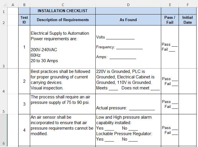
The Users in my department will be hiding and adding rows as needed that already are numbered, so the number column has to handle being Hidden, not Deleted, they may want to UnHide them as needed, so the effort has to recognize hidden rows and then pick up where the last Visible row left off. similar to =SUBTOTAL(102, which skips counting hidden rows, but dont be constrained by using that formula.

I have a long list of items in a range of rows, one per line, which are already numbered,

I have the rows already numbered that matches the VISIBLE rows in about 50 lines.

(by numbered I mean based on which way to go with this, they are actual numbers,

or formulas to dynamically put the next number in place in case any rows get HIDDEN,

like using =AGGREGATE(2,5,B$2:B6)+1 or =SUBTOTAL(102, .....)

Either way is fine with me, and works, until I "Insert a copied row", or adding a row, and the copied row

will not update the AGGREGATE code which has become the problem.

The users using this wont know code or formulas, so I cant expect them to fix it or update it just because they add or copy a row.

This worked great when all they did was click one of my buttons that hid any row they didnt want, its just when a row was Inserted copied row, or added, since the user wont know how to add code to that new row.

There will be at times a row(s) that gets hidden on purpose by the user, not deleted, in this group of rows, and all works fine.

Its just the Insert Copied Row, or them Adding a row, that is my problem.

If I dont use any formula, and the numbers are just Hard entered, 1,2,3,4... I know I can just

select the top 2 numbers and double-click the bottom-right small green square and all the numbers will

run down and be correct.

I know that will work, but Im creating this for non-excel type people who just want to hit a button and let that do it for them.

I didnt need a Button for this until the Insert Copied Cell question was requested, and I still wont need a Button if anyone knows a way

for the number column to auto-renumber by itself based on Hide or Insert Copied cell.

I already have a button and a Macro created for this, but cant find the right combination of code to make it work, when the inserted copied code is used.

Ive tried to use a Counter for items in the description rows that would tell me how many rows there are THAT IS NOT HIDDEN, (AGGREGATE and SUBTOTAL) and use that as a variable to place in a RANGE to re-number the VISIBLE rows, but lack the knowledge how to place that variable in the second part of the range thats always changing, base on if the user has hidden or inserted any rows in this list.

I recorded a Macro to see how Excel handles the 'Select the first 2 rows and click on that bottom-right item to renumber',

and it works, but the range is fixed for that situation, ("B3:B54"), and when a row(s) gets added, I dont know how to increment that last

number to match the new number of rows in my group of rows to renumber.

' Range("B3:B4").Select
' Selection.AutoFill Destination:=Range("B3:B54")
' Range("B3:B54").Select

Ive replaced B54 with the counter variable, but seems to be a mis-match of code and it didnt like that.

Watched several videos, but cant find the right situation. Been several days trying to find a solution.

Tried this too, but a mis-match type error popped-up:

' Selection.AutoFill Destination:=Range("B" & BeginCount & ":B" & TotalRowsToPrint)

If there is a simpler way to approach this, I'll take it.

Anyone with ideas please? Thanks.

Answer 1

BrainStain00,

So you want to number column B not column A.

And the start is in row 3 not row 2.

Edit the named range GroupedRows so that the referenced range is:

=OFFSET(InstallationChklst!$B$2:$F$2,1,0,COUNTA(InstallationChklst!$C:$C)-1)

Put this code in the module of sheet InstallationChklst.

Only then the code will fire when a cell in column B (now not A as before) is changed.

Private Sub Worksheet_Change(ByVal Target As Range)

    Dim rng As Range

    Set rng = ThisWorkbook.Sheets("InstallationChklst").Range("GroupedRows").Columns(1)

    If Not Intersect(Target, rng) Is Nothing Then

        Application.EnableEvents = False

        rng.Formula = "=SubTotal(103,$C$3:C3)"

        Application.EnableEvents = True

    End If

End Sub

Change something in the first column of GroupedRows and that column will be filled with the right formula to number the rows.

I’ve assumed that column C from GroupedRows has a value in every cell (so there is no empty cell in that range) otherwise the numbering is not right.

Jan

Answer 2

My pleasure.

Answer 3

Hi Jan,

Wanted to update you on what I've learned.

First, I needed to add this ability to other sheets in my tool I'm creating,

so your knowledge and help allowed me to now do this, thanks.

So in that successful process, I learned what minor tweaks I needed to do where,

such as in the macro for that sheet, the starting position needs to match the code in each row.

I had one that started lower, like row 12, but didn't change the code in the macro, and it (being a live code),

tried to modify starting at row 3 or 4, and I couldn't figure it out.

So going thru the code at all 3 places, (the actual cells, the macro, and the name manager), I found what to do, and it works.

Also, in adding it to another sheet now, I did not see that extra row number at the end, like the original attempt, odd.

I think its possibly because when I extended the code down in the sheet itself, I may have dragged the code down 1 row too far.

And the reason I couldn't delete it was because the macro is a living code (at least I'm calling it that, because its running on its own).

So this morning I went back to try to learn whats the difference, if any, in all the code in 3 places.

Didn't find any errors, but, did notice in trying to re-drag the code down again from nothing, (deleting the code totally in each row first),

that I could not delete any of it, just like the last row that I couldn't delete, (remember I turned the cell text to white to hide it, lol).

I was able to delete the code in Column B at some point, maybe I had not awakened the sleeping giant, but something triggered it,

and after that I couldn't delete it again after I put it back.

I even closed the file, and re-opened it, but could not immediately delete the contents in Column B, odd.

Because all that code was living code, from the macro.

So what I did, I went to the macro, ' remarked out all the lines with the single quote keystroke, and now the code stopped breathing, lol.

I could delete any rows code and it didn't come back. So I was able to delete all the code in column B, =SUBTOTAL(103,$C$3:C3) as was in B3.

and reinsert it in B3, drag it down 'carefully' to the last row with content in column C, unremark the macro code, and all is perfect now,

nothing beyond the last row with content in column C.

Amazing!!

Anyway, just wanted to pass on the little I learned from using your code, now I can use this will a little more confidence on other sheets in the workbook.

Have a great day Jan.