VBA Code to Automate vlookup based on condition and additional formula.

Question

Hi All

I have recorded a macro to do the following, but it doesn't look neat and creates format issues with unsightly cell data in two columns. Can you possibly assist.

Workbook name = STOCK TAKE AUTOMATION TEMPLATE

The above is the main sheet. VBA should function in the following sequence. The range is Column E3, up to line E78.

(Step 1) If cell E3 has a value, then the value should be deleted and a VLOOKUP formula should be inserted. The lookup value is from Column B.
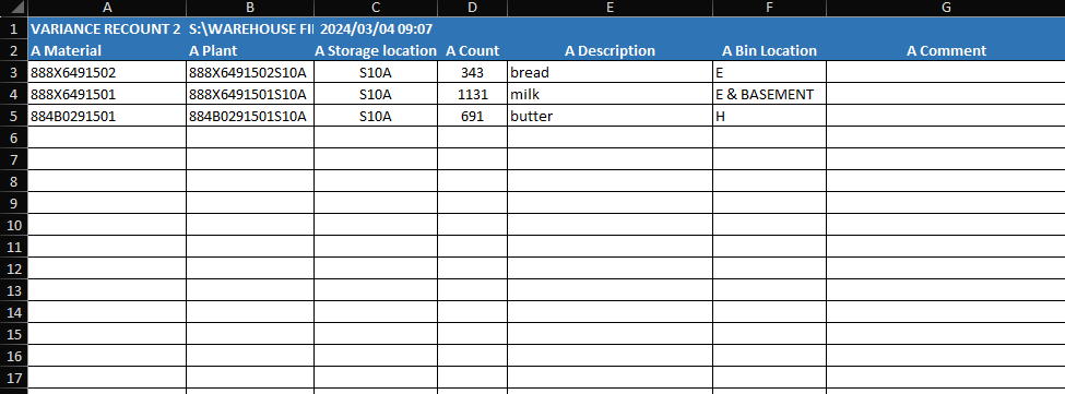
The reference/table is Column B-D in the below workbook. I have the code already that opens that workbook, so it will be visible. The return value is from below column D. See below workbook. This should only be done If range of cells E3 to E78 in STOCK TAKE AUTOMATION TEMPLATE has a value, otherwise nothing should be done.

Workbook name = VARIANCE RECOUNT 2 TEMPLATE

(Step 2) If cells in column G of STOCK TAKE AUTOMATION TEMPLATE has a value, then the value should be deleted, and formula =E3-F3 should be inserted.

I have recorded a macro myself doing the steps, and it works, but the rows with no data, in the range column E & G then has zero values, which creates a problem when I do a print to PDF. See below. So the macro and the way I have approached it works, but the result leaves unsightly cells with formulas included in the PDF print which I would like to avoid, See below.

The end result should look like this:

Any assistance will be greatly appreciated.

Regards

Answer 1

Try this:

Sub Test()
    Dim wst As Worksheet
    Dim r As Long
    Dim m As Long
    Application.ScreenUpdating = False
    Set wst = Worksheets("STOCK TAKE AUTOMATION TEMPLATE")
    m = wst.Range("E" & wst.Rows.Count).End(xlUp).Row
    For r = 2 To m
        If wst.Range("E" & r).Value <> "" Then
            wst.Range("E" & r).FormulaR1C1 = "=VLOOKUP(RC2, 'VARIANCE RECOUNT 2 TEMPLATE'!C2:C4, 3, FALSE)"
            wst.Range("G" & r).FormulaR1C1 = "=RC5-RC6"
        End If
    Next r
    Application.ScreenUpdating = True
End Sub

Answer 2

Hi HansV

Thank you for the response.

I forget to mention the workbook STOCK TAKE AUTOMATION TEMPLATE, has multiple sheets. The sheet applicable is "VARIANCE RECOUNT 2"

The second workbook "VARIANCE RECOUNT 2 TEMPLATE", only has one sheet, which is also called VARIANCE RECOUNT 2. So it's two different workbooks, but the sheets in question for both workbooks have the same sheet name.

Will that change how the above code will works?

Regards

Eugene

Answer 3

Change the line

    Set wst = Worksheets("STOCK TAKE AUTOMATION TEMPLATE")

to

    Set wst = Workbooks("STOCK TAKE AUTOMATION TEMPLATE.xlsx").Worksheets("VARIANCE RECOUNT 2")

Answer 4

Hi Hans

I'm getting the below error:

Answer 5

Can't you place both worksheets in the same workbook? That would make it a lot easier.