invoice/order sheet

Question

Hi I have created a order sheet and invoice, I am trying to set it up so when we enter qty on the order sheet, it reflects onto invoice. I only want it to show the items that have been ordered and not list every item, I have used IFERROR('ORDER SHEET'!C12:F83,5). Is this possible?

Answer 1

Dear @Rebecca,

Based on your description, the approach you’re currently using with IFERROR('ORDER SHEET'!C12:F83,5) will pull all rows from the order sheet, including empty ones, so it won’t meet your requirement of only showing items that have been ordered.

To achieve this, since you want to use a formula that filters the data based on the quantity entered. If you are using a recent version of Excel (Microsoft 365 or Excel 2021), the most effective method is to use the FILTER function. This allows you to dynamically return only the rows where a condition is met, for example, where the quantity is greater than zero.

For more information, you can refer to this Microsoft Official Article here: FILTER function

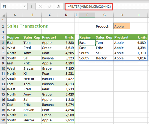
For example, you can use the formula =FILTER(A5:D20,C5:C20=H2,"") to return all records for Apple, as selected in cell H2, and if there are no apples, return an empty string ("").

Additionally, here are some examples you can look through:

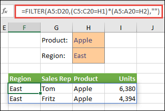
1/ FILTER used to return multiple criteria

In this case, we're using the multiplication operator () to return all values in our array range (A5:D20) that have Apples AND are in the East region: =FILTER(A5:D20,(C5:C20=H1)(A5:A20=H2),"").

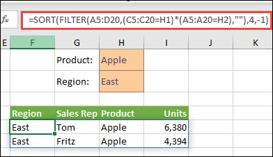
2/ FILTER used to return multiple criteria and sort

In this case, we're using the previous FILTER function with the SORT function to return all values in our array range (A5:D20) that have Apples AND are in the East region, and then sort Units in descending order: =SORT(FILTER(A5:D20,(C5:C20=H1)*(A5:A20=H2),""),4,-1)

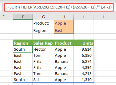
In this case, you can use the FILTER function with the addition operator (+) to return all values in our array range (A5:D20) that have Apples OR are in the East region, and then sort Units in descending order: =SORT(FILTER(A5:D20,(C5:C20=H1)+(A5:A20=H2),""),4,-1).

In the meantime, could you please confirm these questions below to help me diagnose the issue more effectively.

• Could you please confirm where the invoice is located?
• Is the invoice within the same Excel file, or is it stored in another system or application?I hope the information shared helps point you in the right direction. Please try the steps above and let me know if they work. If not, we can continue working together to narrow this down.

The first response may not always resolve the issue right away, but with your help and more details, we can work toward a solution.

Thank you for your patience and understanding. I'm looking forward for your reply.

---

If the answer is helpful, please click "Accept Answer" and kindly upvote it. If you have extra questions about this answer, please click "Comment".   

Note: Please follow the steps in our documentation to enable e-mail notifications if you want to receive the related email notification for this thread.

Answer 2

Use a formula that returns only the ordered items instead of pulling the whole range with IFERROR.

The IFERROR function is meant to catch errors in another formula, not to filter rows. A typical pattern is:

=IFERROR(A2/B2, "Error in calculation")

In this pattern, IFERROR checks the first argument (here A2/B2). If that calculation errors (for example, divide by zero), it returns the second argument; otherwise it returns the calculation result.

To show only items with a quantity on the invoice:

1. On the invoice sheet, in the first item row, use a row-by-row formula that checks the quantity from the order sheet, for example:

      =IF('ORDER SHEET'!C12>0, 'ORDER SHEET'!C12, "")
   

   and similar formulas for description, price, etc.
2. If there is a chance of errors (for example, missing cells or invalid references), wrap the calculation in IFERROR, for example:

      =IFERROR(IF('ORDER SHEET'!C12>0, 'ORDER SHEET'!C12, ""), "")
   

This way, only rows with a quantity greater than zero will show on the invoice; other rows will appear blank instead of listing every item.

---

References:

• IFERROR function