Project Management with Excel - Building a schedule
Are you ready for an intermediate Excel project? This one is fun, very useful, and will teach you a number of handy formulas for manipulating dates in Excel.
I recently had to build a schedule and, in the process, developed a great little system that calculates your dates based on the number of working days needed for each step.
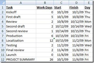
The finished schedule looks like this:
The first thing you need to do is outline your task list and the number of work days required for each step. Also, go ahead and enter all of your column headers.
Once you have this, enter the kickoff date in C2. For D2, enter =WORKDAY(C2,B2) - be sure to format the cells in the Start and Finish columns as Dates, or you may see some strange numeric results instead.
Note that I entered zero for the number of days required to kick off the project since this is mainly just where I enter my start date. If you have a kickoff process and want to count that time, feel free to enter whatever number of days this requires. The great thing about this schedule is how flexible it is!
For E2, enter =TEXT(WEEKDAY(D2), "ddd") to display the day of the week that the step finishes, which I find very handy - particularly if dates move around, as they frequently do, and my boss asks when we are launching.
Next, move down to C3 and enter =D2 to carry down the previous row's finish date, which is the key to making your schedule update dynamically. Finally, copy or fill the remainder of columns C, D, and E down to the final task row (we'll do the PROJECT SUMMARY row in a minute). If you don't have any steps that run at the same time, your schedule should be more or less complete.
In my example above, look at row 8. The Localization step happens in parallel with Production so they share the same Start date ( =D6 in my example). That green mark in C8 indicates that the formula is inconsistent, which is correct here. Just make sure that the finish date for the longest of the parallel steps feeds the start date for the steps that follow.
Now that our schedule is complete, let's add a summary row.
First enter your dates: Start is =C2 and Finish is the launch date, in this case =D11. Then, to calculate the total number of Work Days for the entire project, use =(NETWORKDAYS(C12,D12)-1) - substituting whatever row number you're on for the 12s since your number of tasks may be different from mine. Note: Since the kickoff date and launch date are typically partial days, I subtracted one from the result to more accurately represent the total work time required.
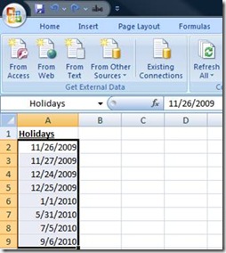
If you want to exclude holidays as part of your working day calculations, there are a few extra steps required. To the right of your main schedule or on a separate tab of the same document, create a column called Holidays where you'll list any holiday dates where your offices are closed that fall within your project dates (to make your schedule re-usable, you may want to enter upcoming holidays for the next 12 months or so). I put mine on a separate tab and entered the last holiday date in my list as part of the tab name.
To quickly find upcoming holidays on your Outlook calendar, go to View, Current View and select Events. Items that are holidays on your calendar will have Holiday in the Categories column.
Now enter any dates that your offices are closed in your schedule document, and then select only the cells with dates. At the top left next to the formula bar is a box that, if you hover over it, says it is called the Name Bar. Type Holidays followed by Enter (NOT Tab!) to save the name for this range of cells:
If you need to edit the range of cells included in a Name (say, to add more holiday dates), click the Formulas tab and then Name Manager.
Now, to exclude these dates, you need to modify a few formulas to recognize your holidays. Go back to your schedule and change D2 to be =WORKDAY(C2,B2,Holidays) and then fill down this row (exclude the summary row; if you get a circular reference warning, you've gone one line too far!). Next, go to your Project Summary Work Days cell (B12 in my example) and change it to =(NETWORKDAYS(C12,D12,Holidays)-1) - again changing the 12s to whatever row you are on in your schedule.
There, your schedule is complete and can easily be maintained during the project by adjusting the number of work days required for a task or replacing the finish date formula with the actual date a task ended. For instance, if Review in my example required an extra day, I could change the Work Days to 3 or simply edit the Finish Date to 10/13/09. The rest of the dates below will be pushed out so that my new end date is 11/9/09.
Told you this was fun! At least as much fun as you can have maintaining a schedule. Just wait until we make our first Gantt chart together…
Suzanne

