Different ways to run the Resource Estimator
In this article, you learn to work with the Azure Quantum Resource Estimator. The Resource Estimator helps you estimate the resources required to run a quantum program on a quantum computer. You can use the Resource Estimator to estimate the number of qubits, the number of gates, and the depth of the circuit required to run a quantum program.
The Resource Estimator is available in Visual Studio Code with the Quantum Development Kit extension. For more information, see Install the Quantum Development Kit.
Warning
The Resource Estimator in Azure portal is deprecated. We recommend that you transition to the local Resource Estimator in Visual Studio Code provided in the Quantum Development Kit.
Prerequisites for VS Code
- The latest version of Visual Studio Code or open VS Code on the Web.
- The latest version of the Quantum Development Kit extension. For installation details, see Installing the QDK on VS Code.
Tip
You don't need to have an Azure account to run the Resource Estimator.
Create a new Q# file
- Open Visual Studio Code and select File > New Text File to create a new file.
- Save the file as
ShorRE.qs. This file will contain the Q# code for your program.
Create the quantum algorithm
Copy the following code into the ShorRE.qs file:
    import Std.Arrays.*;
    import Std.Canon.*;
    import Std.Convert.*;
    import Std.Diagnostics.*;
    import Std.Math.*;
    import Std.Measurement.*;
    import Microsoft.Quantum.Unstable.Arithmetic.*;
    import Std.ResourceEstimation.*;

    operation Main() : Unit {
        let bitsize = 31;

        // When choosing parameters for `EstimateFrequency`, make sure that
        // generator and modules are not co-prime
        let _ = EstimateFrequency(11, 2^bitsize - 1, bitsize);
    }

    // In this sample we concentrate on costing the `EstimateFrequency`
    // operation, which is the core quantum operation in Shors algorithm, and
    // we omit the classical pre- and post-processing.

    /// # Summary
    /// Estimates the frequency of a generator
    /// in the residue ring Z mod `modulus`.
    ///
    /// # Input
    /// ## generator
    /// The unsigned integer multiplicative order (period)
    /// of which is being estimated. Must be co-prime to `modulus`.
    /// ## modulus
    /// The modulus which defines the residue ring Z mod `modulus`
    /// in which the multiplicative order of `generator` is being estimated.
    /// ## bitsize
    /// Number of bits needed to represent the modulus.
    ///
    /// # Output
    /// The numerator k of dyadic fraction k/2^bitsPrecision
    /// approximating s/r.
    operation EstimateFrequency(
        generator : Int,
        modulus : Int,
        bitsize : Int
    )
    : Int {
        mutable frequencyEstimate = 0;
        let bitsPrecision =  2 * bitsize + 1;

        // Allocate qubits for the superposition of eigenstates of
        // the oracle that is used in period finding.
        use eigenstateRegister = Qubit[bitsize];

        // Initialize eigenstateRegister to 1, which is a superposition of
        // the eigenstates we are estimating the phases of.
        // We first interpret the register as encoding an unsigned integer
        // in little endian encoding.
        ApplyXorInPlace(1, eigenstateRegister);
        let oracle = ApplyOrderFindingOracle(generator, modulus, _, _);

        // Use phase estimation with a semiclassical Fourier transform to
        // estimate the frequency.
        use c = Qubit();
        for idx in bitsPrecision - 1..-1..0 {
            within {
                H(c);
            } apply {
                // `BeginEstimateCaching` and `EndEstimateCaching` are the operations
                // exposed by Azure Quantum Resource Estimator. These will instruct
                // resource counting such that the if-block will be executed
                // only once, its resources will be cached, and appended in
                // every other iteration.
                if BeginEstimateCaching("ControlledOracle", SingleVariant()) {
                    Controlled oracle([c], (1 <<< idx, eigenstateRegister));
                    EndEstimateCaching();
                }
                R1Frac(frequencyEstimate, bitsPrecision - 1 - idx, c);
            }
            if MResetZ(c) == One {
                set frequencyEstimate += 1 <<< (bitsPrecision - 1 - idx);
            }
        }

        // Return all the qubits used for oracles eigenstate back to 0 state
        // using Microsoft.Quantum.Intrinsic.ResetAll.
        ResetAll(eigenstateRegister);

        return frequencyEstimate;
    }

    /// # Summary
    /// Interprets `target` as encoding unsigned little-endian integer k
    /// and performs transformation |k⟩ ↦ |gᵖ⋅k mod N ⟩ where
    /// p is `power`, g is `generator` and N is `modulus`.
    ///
    /// # Input
    /// ## generator
    /// The unsigned integer multiplicative order ( period )
    /// of which is being estimated. Must be co-prime to `modulus`.
    /// ## modulus
    /// The modulus which defines the residue ring Z mod `modulus`
    /// in which the multiplicative order of `generator` is being estimated.
    /// ## power
    /// Power of `generator` by which `target` is multiplied.
    /// ## target
    /// Register interpreted as little endian encoded which is multiplied by
    /// given power of the generator. The multiplication is performed modulo
    /// `modulus`.
    internal operation ApplyOrderFindingOracle(
        generator : Int, modulus : Int, power : Int, target : Qubit[]
    )
    : Unit
    is Adj + Ctl {
        // The oracle we use for order finding implements |x⟩ ↦ |x⋅a mod N⟩. We
        // also use `ExpModI` to compute a by which x must be multiplied. Also
        // note that we interpret target as unsigned integer in little-endian
        // encoding.
        ModularMultiplyByConstant(modulus,
                                    ExpModI(generator, power, modulus),
                                    target);
    }

    /// # Summary
    /// Performs modular in-place multiplication by a classical constant.
    ///
    /// # Description
    /// Given the classical constants `c` and `modulus`, and an input
    /// quantum register  |𝑦⟩, this operation
    /// computes `(c*x) % modulus` into |𝑦⟩.
    ///
    /// # Input
    /// ## modulus
    /// Modulus to use for modular multiplication
    /// ## c
    /// Constant by which to multiply |𝑦⟩
    /// ## y
    /// Quantum register of target
    internal operation ModularMultiplyByConstant(modulus : Int, c : Int, y : Qubit[])
    : Unit is Adj + Ctl {
        use qs = Qubit[Length(y)];
        for (idx, yq) in Enumerated(y) {
            let shiftedC = (c <<< idx) % modulus;
            Controlled ModularAddConstant([yq], (modulus, shiftedC, qs));
        }
        ApplyToEachCA(SWAP, Zipped(y, qs));
        let invC = InverseModI(c, modulus);
        for (idx, yq) in Enumerated(y) {
            let shiftedC = (invC <<< idx) % modulus;
            Controlled ModularAddConstant([yq], (modulus, modulus - shiftedC, qs));
        }
    }

    /// # Summary
    /// Performs modular in-place addition of a classical constant into a
    /// quantum register.
    ///
    /// # Description
    /// Given the classical constants `c` and `modulus`, and an input
    /// quantum register  |𝑦⟩, this operation
    /// computes `(x+c) % modulus` into |𝑦⟩.
    ///
    /// # Input
    /// ## modulus
    /// Modulus to use for modular addition
    /// ## c
    /// Constant to add to |𝑦⟩
    /// ## y
    /// Quantum register of target
    internal operation ModularAddConstant(modulus : Int, c : Int, y : Qubit[])
    : Unit is Adj + Ctl {
        body (...) {
            Controlled ModularAddConstant([], (modulus, c, y));
        }
        controlled (ctrls, ...) {
            // We apply a custom strategy to control this operation instead of
            // letting the compiler create the controlled variant for us in which
            // the `Controlled` functor would be distributed over each operation
            // in the body.
            //
            // Here we can use some scratch memory to save ensure that at most one
            // control qubit is used for costly operations such as `AddConstant`
            // and `CompareGreaterThenOrEqualConstant`.
            if Length(ctrls) >= 2 {
                use control = Qubit();
                within {
                    Controlled X(ctrls, control);
                } apply {
                    Controlled ModularAddConstant([control], (modulus, c, y));
                }
            } else {
                use carry = Qubit();
                Controlled AddConstant(ctrls, (c, y + [carry]));
                Controlled Adjoint AddConstant(ctrls, (modulus, y + [carry]));
                Controlled AddConstant([carry], (modulus, y));
                Controlled CompareGreaterThanOrEqualConstant(ctrls, (c, y, carry));
            }
        }
    }

    /// # Summary
    /// Performs in-place addition of a constant into a quantum register.
    ///
    /// # Description
    /// Given a non-empty quantum register |𝑦⟩ of length 𝑛+1 and a positive
    /// constant 𝑐 < 2ⁿ, computes |𝑦 + c⟩ into |𝑦⟩.
    ///
    /// # Input
    /// ## c
    /// Constant number to add to |𝑦⟩.
    /// ## y
    /// Quantum register of second summand and target; must not be empty.
    internal operation AddConstant(c : Int, y : Qubit[]) : Unit is Adj + Ctl {
        // We are using this version instead of the library version that is based
        // on Fourier angles to show an advantage of sparse simulation in this sample.

        let n = Length(y);
        Fact(n > 0, "Bit width must be at least 1");

        Fact(c >= 0, "constant must not be negative");
        Fact(c < 2 ^ n, $"constant must be smaller than {2L ^ n}");

        if c != 0 {
            // If c has j trailing zeroes than the j least significant bits
            // of y won't be affected by the addition and can therefore be
            // ignored by applying the addition only to the other qubits and
            // shifting c accordingly.
            let j = NTrailingZeroes(c);
            use x = Qubit[n - j];
            within {
                ApplyXorInPlace(c >>> j, x);
            } apply {
                IncByLE(x, y[j...]);
            }
        }
    }

    /// # Summary
    /// Performs greater-than-or-equals comparison to a constant.
    ///
    /// # Description
    /// Toggles output qubit `target` if and only if input register `x`
    /// is greater than or equal to `c`.
    ///
    /// # Input
    /// ## c
    /// Constant value for comparison.
    /// ## x
    /// Quantum register to compare against.
    /// ## target
    /// Target qubit for comparison result.
    ///
    /// # Reference
    /// This construction is described in [Lemma 3, arXiv:2201.10200]
    internal operation CompareGreaterThanOrEqualConstant(c : Int, x : Qubit[], target : Qubit)
    : Unit is Adj+Ctl {
        let bitWidth = Length(x);

        if c == 0 {
            X(target);
        } elif c >= 2 ^ bitWidth {
            // do nothing
        } elif c == 2 ^ (bitWidth - 1) {
            ApplyLowTCNOT(Tail(x), target);
        } else {
            // normalize constant
            let l = NTrailingZeroes(c);

            let cNormalized = c >>> l;
            let xNormalized = x[l...];
            let bitWidthNormalized = Length(xNormalized);
            let gates = Rest(IntAsBoolArray(cNormalized, bitWidthNormalized));

            use qs = Qubit[bitWidthNormalized - 1];
            let cs1 = [Head(xNormalized)] + Most(qs);
            let cs2 = Rest(xNormalized);

            within {
                for i in IndexRange(gates) {
                    (gates[i] ? ApplyAnd | ApplyOr)(cs1[i], cs2[i], qs[i]);
                }
            } apply {
                ApplyLowTCNOT(Tail(qs), target);
            }
        }
    }

    /// # Summary
    /// Internal operation used in the implementation of GreaterThanOrEqualConstant.
    internal operation ApplyOr(control1 : Qubit, control2 : Qubit, target : Qubit) : Unit is Adj {
        within {
            ApplyToEachA(X, [control1, control2]);
        } apply {
            ApplyAnd(control1, control2, target);
            X(target);
        }
    }

    internal operation ApplyAnd(control1 : Qubit, control2 : Qubit, target : Qubit)
    : Unit is Adj {
        body (...) {
            CCNOT(control1, control2, target);
        }
        adjoint (...) {
            H(target);
            if (M(target) == One) {
                X(target);
                CZ(control1, control2);
            }
        }
    }


    /// # Summary
    /// Returns the number of trailing zeroes of a number
    ///
    /// ## Example
    /// ```qsharp
    /// let zeroes = NTrailingZeroes(21); // = NTrailingZeroes(0b1101) = 0
    /// let zeroes = NTrailingZeroes(20); // = NTrailingZeroes(0b1100) = 2
    /// ```
    internal function NTrailingZeroes(number : Int) : Int {
        mutable nZeroes = 0;
        mutable copy = number;
        while (copy % 2 == 0) {
            set nZeroes += 1;
            set copy /= 2;
        }
        return nZeroes;
    }

    /// # Summary
    /// An implementation for `CNOT` that when controlled using a single control uses
    /// a helper qubit and uses `ApplyAnd` to reduce the T-count to 4 instead of 7.
    internal operation ApplyLowTCNOT(a : Qubit, b : Qubit) : Unit is Adj+Ctl {
        body (...) {
            CNOT(a, b);
        }

        adjoint self;

        controlled (ctls, ...) {
            // In this application this operation is used in a way that
            // it is controlled by at most one qubit.
            Fact(Length(ctls) <= 1, "At most one control line allowed");

            if IsEmpty(ctls) {
                CNOT(a, b);
            } else {
                use q = Qubit();
                within {
                    ApplyAnd(Head(ctls), a, q);
                } apply {
                    CNOT(q, b);
                }
            }
        }

        controlled adjoint self;
    }
Run the Resource Estimator
The Resource Estimator offers six predefined qubit parameters, four of which have gate-based instruction sets and two that have a Majorana instruction set. It also offers two quantum error correction codes, surface_code and floquet_code.
In this example, you run the Resource Estimator using the qubit_gate_us_e3 qubit parameter and the surface_code quantum error correction code.
Select View -> Command Palette, and type “resource” which should bring up the Q#: Calculate Resource Estimates option. You can also click on Estimate from the list of commands displayed right before the
Mainoperation. Select this option to open the Resource Estimator window.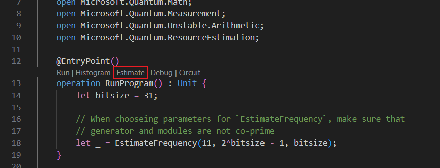
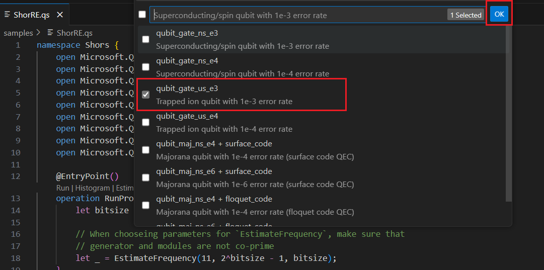
You can select one or more Qubit parameter + Error Correction code types to estimate the resources for. For this example, select qubit_gate_us_e3 and click OK.
Specify the Error budget or accept the default value 0.001. For this example, leave the default value and press Enter.
Press Enter to accept the default result name based on the filename, in this case, ShorRE.
View the results
The Resource Estimator provides multiple estimates for the same algorithm, each showing tradeoffs between the number of qubits and the runtime. Understanding the tradeoff between runtime and system scale is one of the more important aspects of resource estimation.
The result of the resource estimation is displayed in the Q# Estimate window.
The Results tab displays a summary of the resource estimation. Click the icon next to the first row to select the columns you want to display. You can select from run name, estimate type, qubit type, qec scheme, error budget, logical qubits, logical depth, code distance, T states, T factories, T factory fraction, runtime, rQOPS, and physical qubits.
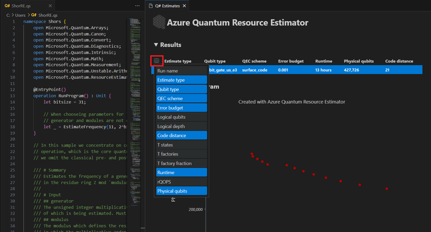
In the Estimate type column of the results table, you can see the number of optimal combinations of {number of qubits, runtime} for your algorithm. These combinations can be seen in the space-time diagram.
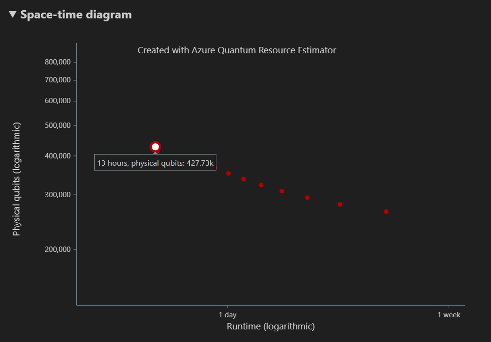
The Space-time diagram shows the tradeoffs between the number of physical qubits and the runtime of the algorithm. In this case, the Resource Estimator finds 13 different optimal combinations out of many thousands possible ones. You can hover over each {number of qubits, runtime} point to see the details of the resource estimation at that point.
For more information, see Space-time diagram.
Note
You need to click on one point of the space-time diagram, that is a {number of qubits, runtime} pair, to see the space diagram and the details of the resource estimation corresponding to that point.
The Space diagram shows the distribution of physical qubits used for the algorithm and the T factories, corresponding to a {number of qubits, runtime} pair. For example, if you select the leftmost point in the space-time diagram, the number of physical qubits required to run the algorithm are 427726, 196686 of which are algorithm qubits and 231040 of which are T factory qubits.
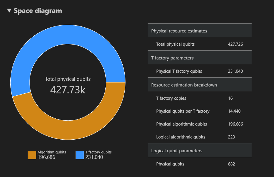
Finally, the Resource Estimates tab displays the full list of output data for the Resource Estimator corresponding to a {number of qubits, runtime} pair. You can inspect cost details by collapsing the groups, which have more information. For example, select the leftmost point in the space-time diagram and collapse the Logical qubit parameters group.
Logical qubit parameter Value QEC scheme surface_code Code distance 21 Physical qubits 882 Logical cycle time 13 millisecs Logical qubit error rate 3.00E-13 Crossing prefactor 0.03 Error correction threshold 0.01 Logical cycle time formula (4 * twoQubitGateTime+ 2 *oneQubitMeasurementTime) *codeDistancePhysical qubits formula 2 * codeDistance*codeDistanceTip
Click Show detailed rows to display the description of each output of the report data.
For more information, see the full report data of the Resource Estimator.
Change the target parameters
You can estimate the cost for the same Q# program using other qubit type, error correction code, and error budget. Open the Resource Estimator window by select View -> Command Palette, and type Q#: Calculate Resource Estimates.
Select any other configuration, for example the Majorana-based qubit parameter, qubit_maj_ns_e6. Accept the default error budget value or enter a new one, and press Enter. The Resource Estimator reruns the estimation with the new target parameters.
For more information, see Target parameters for the Resource Estimator.
Run multiple configurations of parameters
The Azure Quantum Resource Estimator can run multiple configurations of target parameters and compare the resource estimation results.
Select View -> Command Palette, or press Ctrl+Shift+P, and type
Q#: Calculate Resource Estimates.Select qubit_gate_us_e3, qubit_gate_us_e4, qubit_maj_ns_e4 + floquet_code, and qubit_maj_ns_e6 + floquet_code, and click OK.
Accept the default error budget value 0.001 and press Enter.
Press Enter to accept the input file, in this case, ShorRE.qs.
In the case of multiple configurations of parameters, the results are displayed in different rows in the Results tab.
The Space-time diagram shows the results for all the configurations of parameters. The first column of the results table displays the legend for each configuration of parameters. You can hover over each point to see the details of the resource estimation at that point.
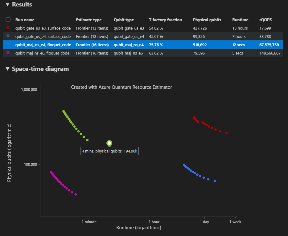
Click on a {number of qubits, runtime} point of the space-time diagram to bring up the corresponding space diagram and report data.
Prerequisites for Jupyter Notebook in VS Code
A Python environment with Python and Pip installed.
The latest version of Visual Studio Code or open VS Code on the Web.
VS Code with the Quantum Development Kit, Python, and Jupyter extensions installed.
The latest Azure Quantum
qsharpandqsharp-widgetspackages.!pip install --upgrade qsharp qsharp-widgets
Tip
You don't need to have an Azure account to run the Resource Estimator.
Create the quantum algorithm
In VS Code, select View > Command palette and select Create: New Jupyter Notebook.
In the top-right, VS Code will detect and display the version of Python and the virtual Python environment that was selected for the notebook. If you have multiple Python environments, you may need to select a kernel using the kernel picker in the top right. If no environment was detected, see Jupyter Notebooks in VS Code for setup information.
In the first cell of the notebook, import the
qsharppackage.import qsharpAdd a new cell and copy the following code.
%%qsharp
import Std.Arrays.*;
import Std.Canon.*;
import Std.Convert.*;
import Std.Diagnostics.*;
import Std.Math.*;
import Std.Measurement.*;
import Microsoft.Quantum.Unstable.Arithmetic.*;
import Std.ResourceEstimation.*;

operation RunProgram() : Unit {
    let bitsize = 31;

    // When choosing parameters for `EstimateFrequency`, make sure that
    // generator and modules are not co-prime
    let _ = EstimateFrequency(11, 2^bitsize - 1, bitsize);
}


// In this sample we concentrate on costing the `EstimateFrequency`
// operation, which is the core quantum operation in Shors algorithm, and
// we omit the classical pre- and post-processing.

/// # Summary
/// Estimates the frequency of a generator
/// in the residue ring Z mod `modulus`.
///
/// # Input
/// ## generator
/// The unsigned integer multiplicative order (period)
/// of which is being estimated. Must be co-prime to `modulus`.
/// ## modulus
/// The modulus which defines the residue ring Z mod `modulus`
/// in which the multiplicative order of `generator` is being estimated.
/// ## bitsize
/// Number of bits needed to represent the modulus.
///
/// # Output
/// The numerator k of dyadic fraction k/2^bitsPrecision
/// approximating s/r.
operation EstimateFrequency(
    generator : Int,
    modulus : Int,
    bitsize : Int
)
: Int {
    mutable frequencyEstimate = 0;
    let bitsPrecision =  2 * bitsize + 1;

    // Allocate qubits for the superposition of eigenstates of
    // the oracle that is used in period finding.
    use eigenstateRegister = Qubit[bitsize];

    // Initialize eigenstateRegister to 1, which is a superposition of
    // the eigenstates we are estimating the phases of.
    // We first interpret the register as encoding an unsigned integer
    // in little endian encoding.
    ApplyXorInPlace(1, eigenstateRegister);
    let oracle = ApplyOrderFindingOracle(generator, modulus, _, _);

    // Use phase estimation with a semiclassical Fourier transform to
    // estimate the frequency.
    use c = Qubit();
    for idx in bitsPrecision - 1..-1..0 {
        within {
            H(c);
        } apply {
            // `BeginEstimateCaching` and `EndEstimateCaching` are the operations
            // exposed by Azure Quantum Resource Estimator. These will instruct
            // resource counting such that the if-block will be executed
            // only once, its resources will be cached, and appended in
            // every other iteration.
            if BeginEstimateCaching("ControlledOracle", SingleVariant()) {
                Controlled oracle([c], (1 <<< idx, eigenstateRegister));
                EndEstimateCaching();
            }
            R1Frac(frequencyEstimate, bitsPrecision - 1 - idx, c);
        }
        if MResetZ(c) == One {
            set frequencyEstimate += 1 <<< (bitsPrecision - 1 - idx);
        }
    }

    // Return all the qubits used for oracle eigenstate back to 0 state
    // using Microsoft.Quantum.Intrinsic.ResetAll.
    ResetAll(eigenstateRegister);

    return frequencyEstimate;
}

/// # Summary
/// Interprets `target` as encoding unsigned little-endian integer k
/// and performs transformation |k⟩ ↦ |gᵖ⋅k mod N ⟩ where
/// p is `power`, g is `generator` and N is `modulus`.
///
/// # Input
/// ## generator
/// The unsigned integer multiplicative order ( period )
/// of which is being estimated. Must be co-prime to `modulus`.
/// ## modulus
/// The modulus which defines the residue ring Z mod `modulus`
/// in which the multiplicative order of `generator` is being estimated.
/// ## power
/// Power of `generator` by which `target` is multiplied.
/// ## target
/// Register interpreted as little endian encoded which is multiplied by
/// given power of the generator. The multiplication is performed modulo
/// `modulus`.
internal operation ApplyOrderFindingOracle(
    generator : Int, modulus : Int, power : Int, target : Qubit[]
)
: Unit
is Adj + Ctl {
    // The oracle we use for order finding implements |x⟩ ↦ |x⋅a mod N⟩. We
    // also use `ExpModI` to compute a by which x must be multiplied. Also
    // note that we interpret target as unsigned integer in little-endian
    // encoding.
    ModularMultiplyByConstant(modulus,
                                ExpModI(generator, power, modulus),
                                target);
}

/// # Summary
/// Performs modular in-place multiplication by a classical constant.
///
/// # Description
/// Given the classical constants `c` and `modulus`, and an input
/// quantum register |𝑦⟩, this operation
/// computes `(c*x) % modulus` into |𝑦⟩.
///
/// # Input
/// ## modulus
/// Modulus to use for modular multiplication
/// ## c
/// Constant by which to multiply |𝑦⟩
/// ## y
/// Quantum register of target
internal operation ModularMultiplyByConstant(modulus : Int, c : Int, y : Qubit[])
: Unit is Adj + Ctl {
    use qs = Qubit[Length(y)];
    for (idx, yq) in Enumerated(y) {
        let shiftedC = (c <<< idx) % modulus;
        Controlled ModularAddConstant([yq], (modulus, shiftedC, qs));
    }
    ApplyToEachCA(SWAP, Zipped(y, qs));
    let invC = InverseModI(c, modulus);
    for (idx, yq) in Enumerated(y) {
        let shiftedC = (invC <<< idx) % modulus;
        Controlled ModularAddConstant([yq], (modulus, modulus - shiftedC, qs));
    }
}

/// # Summary
/// Performs modular in-place addition of a classical constant into a
/// quantum register.
///
/// # Description
/// Given the classical constants `c` and `modulus`, and an input
/// quantum register  |𝑦⟩, this operation
/// computes `(x+c) % modulus` into |𝑦⟩.
///
/// # Input
/// ## modulus
/// Modulus to use for modular addition
/// ## c
/// Constant to add to |𝑦⟩
/// ## y
/// Quantum register of target
internal operation ModularAddConstant(modulus : Int, c : Int, y : Qubit[])
: Unit is Adj + Ctl {
    body (...) {
        Controlled ModularAddConstant([], (modulus, c, y));
    }
    controlled (ctrls, ...) {
        // We apply a custom strategy to control this operation instead of
        // letting the compiler create the controlled variant for us in which
        // the `Controlled` functor would be distributed over each operation
        // in the body.
        //
        // Here we can use some scratch memory to save ensure that at most one
        // control qubit is used for costly operations such as `AddConstant`
        // and `CompareGreaterThenOrEqualConstant`.
        if Length(ctrls) >= 2 {
            use control = Qubit();
            within {
                Controlled X(ctrls, control);
            } apply {
                Controlled ModularAddConstant([control], (modulus, c, y));
            }
        } else {
            use carry = Qubit();
            Controlled AddConstant(ctrls, (c, y + [carry]));
            Controlled Adjoint AddConstant(ctrls, (modulus, y + [carry]));
            Controlled AddConstant([carry], (modulus, y));
            Controlled CompareGreaterThanOrEqualConstant(ctrls, (c, y, carry));
        }
    }
}

/// # Summary
/// Performs in-place addition of a constant into a quantum register.
///
/// # Description
/// Given a non-empty quantum register |𝑦⟩ of length 𝑛+1 and a positive
/// constant 𝑐 < 2ⁿ, computes |𝑦 + c⟩ into |𝑦⟩.
///
/// # Input
/// ## c
/// Constant number to add to |𝑦⟩.
/// ## y
/// Quantum register of second summand and target; must not be empty.
internal operation AddConstant(c : Int, y : Qubit[]) : Unit is Adj + Ctl {
    // We are using this version instead of the library version that is based
    // on Fourier angles to show an advantage of sparse simulation in this sample.

    let n = Length(y);
    Fact(n > 0, "Bit width must be at least 1");

    Fact(c >= 0, "constant must not be negative");
    Fact(c < 2 ^ n, $"constant must be smaller than {2L ^ n}");

    if c != 0 {
        // If c has j trailing zeroes than the j least significant bits
        // of y will not be affected by the addition and can therefore be
        // ignored by applying the addition only to the other qubits and
        // shifting c accordingly.
        let j = NTrailingZeroes(c);
        use x = Qubit[n - j];
        within {
            ApplyXorInPlace(c >>> j, x);
        } apply {
            IncByLE(x, y[j...]);
        }
    }
}

/// # Summary
/// Performs greater-than-or-equals comparison to a constant.
///
/// # Description
/// Toggles output qubit `target` if and only if input register `x`
/// is greater than or equal to `c`.
///
/// # Input
/// ## c
/// Constant value for comparison.
/// ## x
/// Quantum register to compare against.
/// ## target
/// Target qubit for comparison result.
///
/// # Reference
/// This construction is described in [Lemma 3, arXiv:2201.10200]
internal operation CompareGreaterThanOrEqualConstant(c : Int, x : Qubit[], target : Qubit)
: Unit is Adj+Ctl {
    let bitWidth = Length(x);

    if c == 0 {
        X(target);
    } elif c >= 2 ^ bitWidth {
        // do nothing
    } elif c == 2 ^ (bitWidth - 1) {
        ApplyLowTCNOT(Tail(x), target);
    } else {
        // normalize constant
        let l = NTrailingZeroes(c);

        let cNormalized = c >>> l;
        let xNormalized = x[l...];
        let bitWidthNormalized = Length(xNormalized);
        let gates = Rest(IntAsBoolArray(cNormalized, bitWidthNormalized));

        use qs = Qubit[bitWidthNormalized - 1];
        let cs1 = [Head(xNormalized)] + Most(qs);
        let cs2 = Rest(xNormalized);

        within {
            for i in IndexRange(gates) {
                (gates[i] ? ApplyAnd | ApplyOr)(cs1[i], cs2[i], qs[i]);
            }
        } apply {
            ApplyLowTCNOT(Tail(qs), target);
        }
    }
}

/// # Summary
/// Internal operation used in the implementation of GreaterThanOrEqualConstant.
internal operation ApplyOr(control1 : Qubit, control2 : Qubit, target : Qubit) : Unit is Adj {
    within {
        ApplyToEachA(X, [control1, control2]);
    } apply {
        ApplyAnd(control1, control2, target);
        X(target);
    }
}

internal operation ApplyAnd(control1 : Qubit, control2 : Qubit, target : Qubit)
: Unit is Adj {
    body (...) {
        CCNOT(control1, control2, target);
    }
    adjoint (...) {
        H(target);
        if (M(target) == One) {
            X(target);
            CZ(control1, control2);
        }
    }
}


/// # Summary
/// Returns the number of trailing zeroes of a number
///
/// ## Example
/// ```qsharp
/// let zeroes = NTrailingZeroes(21); // = NTrailingZeroes(0b1101) = 0
/// let zeroes = NTrailingZeroes(20); // = NTrailingZeroes(0b1100) = 2
/// ```
internal function NTrailingZeroes(number : Int) : Int {
    mutable nZeroes = 0;
    mutable copy = number;
    while (copy % 2 == 0) {
        set nZeroes += 1;
        set copy /= 2;
    }
    return nZeroes;
}

/// # Summary
/// An implementation for `CNOT` that when controlled using a single control uses
/// a helper qubit and uses `ApplyAnd` to reduce the T-count to 4 instead of 7.
internal operation ApplyLowTCNOT(a : Qubit, b : Qubit) : Unit is Adj+Ctl {
    body (...) {
        CNOT(a, b);
    }

    adjoint self;

    controlled (ctls, ...) {
        // In this application this operation is used in a way that
        // it is controlled by at most one qubit.
        Fact(Length(ctls) <= 1, "At most one control line allowed");

        if IsEmpty(ctls) {
            CNOT(a, b);
        } else {
            use q = Qubit();
            within {
                ApplyAnd(Head(ctls), a, q);
            } apply {
                CNOT(q, b);
            }
        }
    }

    controlled adjoint self;
}
Estimate the quantum algorithm
Now, you estimate the physical resources for the RunProgram operation using the default assumptions. Add a new cell and copy the following code.
result = qsharp.estimate("RunProgram()")
result
The qsharp.estimate function creates a result object, which can be used to display a table with the overall physical resource counts. You can inspect cost details by expanding the groups, which have more information. For more information, see the full report data of the Resource Estimator.
For example, expand the Logical qubit parameters group to see that the code distance is 21 and the number of physical qubits is 882.
| Logical qubit parameter | Value |
|---|---|
| QEC scheme | surface_code |
| Code distance | 21 |
| Physical qubits | 882 |
| Logical cycle time | 8 millisecs |
| Logical qubit error rate | 3.00E-13 |
| Crossing prefactor | 0.03 |
| Error correction threshold | 0.01 |
| Logical cycle time formula | (4 * twoQubitGateTime + 2 * oneQubitMeasurementTime) * codeDistance |
| Physical qubits formula | 2 * codeDistance * codeDistance |
Tip
For a more compact version of the output table, you can use result.summary.
Space diagram
The distribution of physical qubits used for the algorithm and the T factories is a factor which may impact the design of your algorithm. You can use the qsharp-widgets package to visualize this distribution to better understand the estimated space requirements for the algorithm.
from qsharp-widgets import SpaceChart, EstimateDetails
SpaceChart(result)
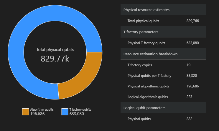
In this example, the number of physical qubits required to run the algorithm are 829766, 196686 of which are algorithm qubits and 633080 of which are T factory qubits.
Change the default values and estimate the algorithm
When submitting a resource estimate request for your program, you can specify some optional parameters. Use the jobParams field to access all the target parameters that can be passed to the job execution and see which default values were assumed:
result['jobParams']
{'errorBudget': 0.001,
 'qecScheme': {'crossingPrefactor': 0.03,
  'errorCorrectionThreshold': 0.01,
  'logicalCycleTime': '(4 * twoQubitGateTime + 2 * oneQubitMeasurementTime) * codeDistance',
  'name': 'surface_code',
  'physicalQubitsPerLogicalQubit': '2 * codeDistance * codeDistance'},
 'qubitParams': {'instructionSet': 'GateBased',
  'name': 'qubit_gate_ns_e3',
  'oneQubitGateErrorRate': 0.001,
  'oneQubitGateTime': '50 ns',
  'oneQubitMeasurementErrorRate': 0.001,
  'oneQubitMeasurementTime': '100 ns',
  'tGateErrorRate': 0.001,
  'tGateTime': '50 ns',
  'twoQubitGateErrorRate': 0.001,
  'twoQubitGateTime': '50 ns'}}
You can see that the Resource Estimator takes the qubit_gate_ns_e3 qubit model, the surface_code error correction code, and 0.001 error budget as default values for the estimation.
These are the target parameters that can be customized:
errorBudget- the overall allowed error budget for the algorithmqecScheme- the quantum error correction (QEC) schemequbitParams- the physical qubit parametersconstraints- the constraints on the component-leveldistillationUnitSpecifications- the specifications for T factories distillation algorithmsestimateType- single or frontier
For more information, see Target parameters for the Resource Estimator.
Change qubit model
You can estimate the cost for the same algorithm using the Majorana-based qubit parameter, qubitParams, "qubit_maj_ns_e6".
result_maj = qsharp.estimate("RunProgram()", params={
                "qubitParams": {
                    "name": "qubit_maj_ns_e6"
                }})
EstimateDetails(result_maj)
Change quantum error correction scheme
You can rerun the resource estimation job for the same example on the Majorana-based qubit parameters with a floqued QEC scheme, qecScheme.
result_maj = qsharp.estimate("RunProgram()", params={
                "qubitParams": {
                    "name": "qubit_maj_ns_e6"
                },
                "qecScheme": {
                    "name": "floquet_code"
                }})
EstimateDetails(result_maj)
Change error budget
Next, rerun the same quantum circuit with an errorBudget of 10%.
result_maj = qsharp.estimate("RunProgram()", params={
                "qubitParams": {
                    "name": "qubit_maj_ns_e6"
                },
                "qecScheme": {
                    "name": "floquet_code"
                },
                "errorBudget": 0.1})
EstimateDetails(result_maj)
Batching with the Resource Estimator
The Azure Quantum Resource Estimator allows you to run multiple configuration of target parameters, and compare the results. This is useful when you want to compare the cost of different qubit models, QEC schemes, or error budgets.
You can perform a batch estimation by passing a list of target parameters to the
paramsparameter of theqsharp.estimatefunction. For example, run the same algorithm with the default parameters and the Majorana-based qubit parameters with a floquet QEC scheme.result_batch = qsharp.estimate("RunProgram()", params= [{}, # Default parameters { "qubitParams": { "name": "qubit_maj_ns_e6" }, "qecScheme": { "name": "floquet_code" } }]) result_batch.summary_data_frame(labels=["Gate-based ns, 10⁻³", "Majorana ns, 10⁻⁶"])Model Logical qubits Logical depth T states Code distance T factories T factory fraction Physical qubits rQOPS Physical runtime Gate-based ns, 10⁻³ 223 3.64M 4.70M 21 19 76.30 % 829.77k 26.55M 31 secs Majorana ns, 10⁻⁶ 223 3.64M 4.70M 5 19 63.02 % 79.60k 148.67M 5 secs You can also construct a list of estimation parameters using the
EstimatorParamsclass.from qsharp.estimator import EstimatorParams, QubitParams, QECScheme, LogicalCounts labels = ["Gate-based µs, 10⁻³", "Gate-based µs, 10⁻⁴", "Gate-based ns, 10⁻³", "Gate-based ns, 10⁻⁴", "Majorana ns, 10⁻⁴", "Majorana ns, 10⁻⁶"] params = EstimatorParams(num_items=6) params.error_budget = 0.333 params.items[0].qubit_params.name = QubitParams.GATE_US_E3 params.items[1].qubit_params.name = QubitParams.GATE_US_E4 params.items[2].qubit_params.name = QubitParams.GATE_NS_E3 params.items[3].qubit_params.name = QubitParams.GATE_NS_E4 params.items[4].qubit_params.name = QubitParams.MAJ_NS_E4 params.items[4].qec_scheme.name = QECScheme.FLOQUET_CODE params.items[5].qubit_params.name = QubitParams.MAJ_NS_E6 params.items[5].qec_scheme.name = QECScheme.FLOQUET_CODEqsharp.estimate("RunProgram()", params=params).summary_data_frame(labels=labels)Model Logical qubits Logical depth T states Code distance T factories T factory fraction Physical qubits rQOPS Physical runtime Gate-based µs, 10⁻³ 223 3.64M 4.70M 17 13 40.54 % 216.77k 21.86k 10 hours Gate-based µs, 10⁻⁴ 223 3.64M 4.70M 9 14 43.17 % 63.57k 41.30k 5 hours Gate-based ns, 10⁻³ 223 3.64M 4.70M 17 16 69.08 % 416.89k 32.79M 25 secs Gate-based ns, 10⁻⁴ 223 3.64M 4.70M 9 14 43.17 % 63.57k 61.94M 13 secs Majorana ns, 10⁻⁴ 223 3.64M 4.70M 9 19 82.75 % 501.48k 82.59M 10 secs Majorana ns, 10⁻⁶ 223 3.64M 4.70M 5 13 31.47 % 42.96k 148.67M 5 secs
Running Pareto frontier estimation
When estimating the resources of an algorithm, it's important to consider the tradeoff between the number of physical qubits and the runtime of the algorithm. You could consider allocation of as many physical qubits as possible to reduce the runtime of the algorithm. However, the number of physical qubits is limited by the number of physical qubits available in the quantum hardware.
The Pareto frontier estimation provides multiple estimates for the same algorithm, each with a tradeoff between the number of qubits and the runtime.
To run the Resource Estimator using Pareto frontier estimation, you need to specify the
"estimateType"target parameter as"frontier". For example, run the same algorithm with the Majorana-based qubit parameters with a surface code using Pareto frontier estimation.result = qsharp.estimate("RunProgram()", params= {"qubitParams": { "name": "qubit_maj_ns_e4" }, "qecScheme": { "name": "surface_code" }, "estimateType": "frontier", # frontier estimation } )You can use the
EstimatesOverviewfunction to display a table with the overall physical resource counts. Click the icon next to the first row to select the columns you want to display. You can select from run name, estimate type, qubit type, qec scheme, error budget, logical qubits, logical depth, code distance, T states, T factories, T factory fraction, runtime, rQOPS, and physical qubits.from qsharp_widgets import EstimatesOverview EstimatesOverview(result)
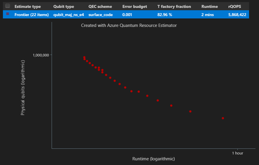
In the Estimate type column of the results table, you can see the number of different combinations of {number of qubits, runtime} for your algorithm. In this case, the Resource Estimator finds 22 different optimal combinations out of many thousands possible ones.
Space-time diagram
The EstimatesOverview function also displays the space-time diagram of the Resource Estimator.
The space-time diagram shows the number of physical qubits and the runtime of the algorithm for each {number of qubits, runtime} pair. You can hover over each point to see the details of the resource estimation at that point.
Batching with Pareto frontier estimation
To estimate and compare multiple configurations of target parameters with frontier estimation, add
"estimateType": "frontier",to the parameters.result = qsharp.estimate( "RunProgram()", [ { "qubitParams": { "name": "qubit_maj_ns_e4" }, "qecScheme": { "name": "surface_code" }, "estimateType": "frontier", # Pareto frontier estimation }, { "qubitParams": { "name": "qubit_maj_ns_e6" }, "qecScheme": { "name": "floquet_code" }, "estimateType": "frontier", # Pareto frontier estimation }, ] ) EstimatesOverview(result, colors=["#1f77b4", "#ff7f0e"], runNames=["e4 Surface Code", "e6 Floquet Code"])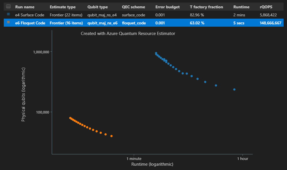
Note
You can define colors and run names for the qubit-time diagram using the
EstimatesOverviewfunction.When running multiple configurations of target parameters using the Pareto frontier estimation, you can see the resource estimates for a specific point of the space-time diagram, that is for each {number of qubits, runtime} pair. For example, the following code shows the estimate details usage for the second (estimate index=0) run and the fourth (point index=3) shortest runtime.
EstimateDetails(result[1], 4)You can also see the space diagram for a specific point of the space-time diagram. For example, the following code shows the space diagram for the first run of combinations (estimate index=0) and the third shortest runtime (point index=2).
SpaceChart(result[0], 2)
Prerequisites for Qiskit in VS Code
A Python environment with Python and Pip installed.
The latest version of Visual Studio Code or open Visual Studio Code on the Web.
VS Code with the Quantum Development Kit, Python, and Jupyter extensions installed.
The latest Azure Quantum
qsharpandqsharp-widgets, andqiskitpackages.!pip install --upgrade qsharp qsharp-widgets qiskit
Tip
You don't need to have an Azure account to run the Resource Estimator.
Create a new Jupyter Notebook
- In VS Code, select View > Command palette and select Create: New Jupyter Notebook.
- In the top-right, VS Code will detect and display the version of Python and the virtual Python environment that was selected for the notebook. If you have multiple Python environments, you may need to select a kernel using the kernel picker in the top right. If no environment was detected, see Jupyter Notebooks in VS Code for setup information.
Create the quantum algorithm
In this example, you create a quantum circuit for a multiplier based on the construction presented in Ruiz-Perez and Garcia-Escartin (arXiv:1411.5949) which uses the Quantum Fourier Transform to implement arithmetic.
You can adjust the size of the multiplier by changing the bitwidth variable. The circuit generation is wrapped in a function that can be called with the bitwidth value of the multiplier. The operation will have two input registers, each the size of the specified bitwidth, and one output register that is twice the size of the specified bitwidth. The function will also print some logical resource counts for the multiplier extracted directly from the quantum circuit.
from qiskit.circuit.library import RGQFTMultiplier

def create_algorithm(bitwidth):
    print(f"[INFO] Create a QFT-based multiplier with bitwidth {bitwidth}")

    circ = RGQFTMultiplier(num_state_qubits=bitwidth)

    return circ
Note
If you select a Python kernel and the qiskit module isn't recognized, try selecting a different Python environment in the kernel picker.
Estimate the quantum algorithm
Create an instance of your algorithm using the create_algorithm function. You can adjust the size of the multiplier by changing the bitwidth variable.
bitwidth = 4

circ = create_algorithm(bitwidth)
Estimate the physical resources for this operation using the default assumptions. You can use the estimate call, which is overloaded to accept a QuantumCircuit object from Qiskit.
from qsharp.estimator import EstimatorParams
from qsharp.interop.qiskit import estimate

params = EstimatorParams()
result = estimate(circ, params)
Alternatively, you can use the ResourceEstimatorBackend to perform the estimation as the existing backend does.
from qsharp.interop.qiskit import ResourceEstimatorBackend
from qsharp.estimator import EstimatorParams

params = EstimatorParams()
backend = ResourceEstimatorBackend()

job = backend.run(circ, params)
result = job.result()
The result object contains the output of the resource estimation job. You can use the EstimateDetails function to display the results in a more readable format.
from qsharp_widgets import EstimateDetails
EstimateDetails(result)
EstimateDetails function displays a table with the overall physical resource counts. You can inspect cost details by expanding the groups, which have more information. For more information, see the full report data of the Resource Estimator.
For example, if you expand the Logical qubit parameters group, you can more easily see that the error correction code distance is 15.
| Logical qubit parameter | Value |
|---|---|
| QEC scheme | surface_code |
| Code distance | 15 |
| Physical qubits | 450 |
| Logical cycle time | 6us |
| Logical qubit error rate | 3.00E-10 |
| Crossing prefactor | 0.03 |
| Error correction threshold | 0.01 |
| Logical cycle time formula | (4 * twoQubitGateTime + 2 * oneQubitMeasurementTime) * codeDistance |
| Physical qubits formula | 2 * codeDistance * codeDistance |
In the Physical qubit parameters group you can see the physical qubit properties that were assumed for this estimation. For example, the time to perform a single-qubit measurement and a single-qubit gate are assumed to be 100 ns and 50 ns, respectively.
Tip
You can also access the output of the Resource Estimator as a Python dictionary using the result.data() method. For example, to access the physical counts result.data()["physicalCounts"].
Space diagrams
The distribution of physical qubits used for the algorithm and the T factories is a factor which may impact the design of your algorithm. You can visualize this distribution to better understand the estimated space requirements for the algorithm.
from qsharp_widgets import SpaceChart

SpaceChart(result)
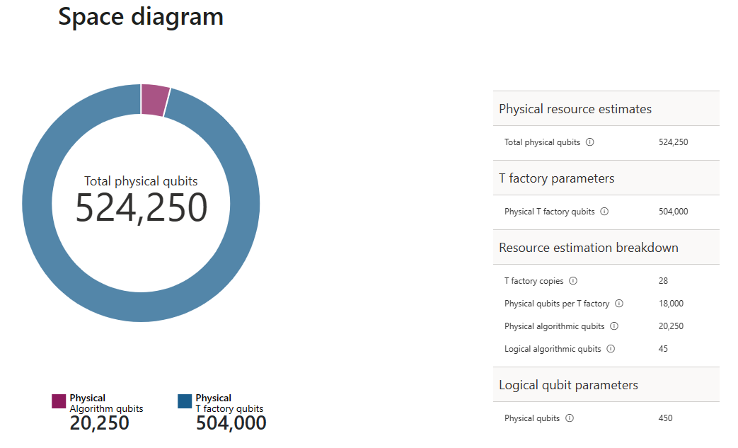
The space diagram shows the proportion of algorithm qubits and T factory qubits. Note that the number of T factory copies, 19, contributes to the number of physical qubits for T factories as $\text{T factories} \cdot \text{physical qubit per T factory}= 19 \cdot 18,000 = 342,000$.
For more information, see T factory physical estimation.
Change the default values and estimate the algorithm
When submitting a resource estimate request for your program, you can specify some optional parameters. Use the jobParams field to access all the values that can be passed to the job execution and see which default values were assumed:
result.data()["jobParams"]
{'errorBudget': 0.001,
 'qecScheme': {'crossingPrefactor': 0.03,
  'errorCorrectionThreshold': 0.01,
  'logicalCycleTime': '(4 * twoQubitGateTime + 2 * oneQubitMeasurementTime) * codeDistance',
  'name': 'surface_code',
  'physicalQubitsPerLogicalQubit': '2 * codeDistance * codeDistance'},
 'qubitParams': {'instructionSet': 'GateBased',
  'name': 'qubit_gate_ns_e3',
  'oneQubitGateErrorRate': 0.001,
  'oneQubitGateTime': '50 ns',
  'oneQubitMeasurementErrorRate': 0.001,
  'oneQubitMeasurementTime': '100 ns',
  'tGateErrorRate': 0.001,
  'tGateTime': '50 ns',
  'twoQubitGateErrorRate': 0.001,
  'twoQubitGateTime': '50 ns'}}
These are the target parameters that can be customized:
errorBudget- the overall allowed error budgetqecScheme- the quantum error correction (QEC) schemequbitParams- the physical qubit parametersconstraints- the constraints on the component-leveldistillationUnitSpecifications- the specifications for T factories distillation algorithms
For more information, see Target parameters for the Resource Estimator.
Change qubit model
Next, estimate the cost for the same algorithm using the Majorana-based qubit parameter qubit_maj_ns_e6
qubitParams = {
    "name": "qubit_maj_ns_e6"
}

result = backend.run(circ, qubitParams).result()
You can inspect the physical counts programmatically. For example, you can explore details about the T factory that was created to execute the algorithm.
result.data()["tfactory"]
{'eccDistancePerRound': [1, 1, 5],
 'logicalErrorRate': 1.6833177305222897e-10,
 'moduleNamePerRound': ['15-to-1 space efficient physical',
  '15-to-1 RM prep physical',
  '15-to-1 RM prep logical'],
 'numInputTstates': 20520,
 'numModulesPerRound': [1368, 20, 1],
 'numRounds': 3,
 'numTstates': 1,
 'physicalQubits': 16416,
 'physicalQubitsPerRound': [12, 31, 1550],
 'runtime': 116900.0,
 'runtimePerRound': [4500.0, 2400.0, 110000.0]}
Note
By default, runtime is shown in nanoseconds.
You can use this data to produce some explanations of how the T factories produce the required T states.
data = result.data()
tfactory = data["tfactory"]
breakdown = data["physicalCounts"]["breakdown"]
producedTstates = breakdown["numTfactories"] * breakdown["numTfactoryRuns"] * tfactory["numTstates"]

print(f"""A single T factory produces {tfactory["logicalErrorRate"]:.2e} T states with an error rate of (required T state error rate is {breakdown["requiredLogicalTstateErrorRate"]:.2e}).""")
print(f"""{breakdown["numTfactories"]} copie(s) of a T factory are executed {breakdown["numTfactoryRuns"]} time(s) to produce {producedTstates} T states ({breakdown["numTstates"]} are required by the algorithm).""")
print(f"""A single T factory is composed of {tfactory["numRounds"]} rounds of distillation:""")
for round in range(tfactory["numRounds"]):
    print(f"""- {tfactory["numUnitsPerRound"][round]} {tfactory["unitNamePerRound"][round]} unit(s)""")
A single T factory produces 1.68e-10 T states with an error rate of (required T state error rate is 2.77e-08).
23 copies of a T factory are executed 523 time(s) to produce 12029 T states (12017 are required by the algorithm).
A single T factory is composed of 3 rounds of distillation:
- 1368 15-to-1 space efficient physical unit(s)
- 20 15-to-1 RM prep physical unit(s)
- 1 15-to-1 RM prep logical unit(s)
Change quantum error correction scheme
Now, rerun the resource estimation job for the same example on the Majorana-based qubit parameters with a floqued QEC scheme, qecScheme.
params = {
    "qubitParams": {"name": "qubit_maj_ns_e6"},
    "qecScheme": {"name": "floquet_code"}
}

result_maj_floquet = backend.run(circ, params).result()
EstimateDetails(result_maj_floquet)
Change error budget
Let's rerun the same quantum circuit with an errorBudget of 10%.
params = {
    "errorBudget": 0.01,
    "qubitParams": {"name": "qubit_maj_ns_e6"},
    "qecScheme": {"name": "floquet_code"},
}
result_maj_floquet_e1 = backend.run(circ, params).result()
EstimateDetails(result_maj_floquet_e1)
Note
If you run into any issue while working with the Resource Estimator, check out the Troubleshooting page, or contact AzureQuantumInfo@microsoft.com.