Note
Access to this page requires authorization. You can try signing in or changing directories.
Access to this page requires authorization. You can try changing directories.
This tutorial shows how to write and simulate a basic quantum program that operates on individual qubits.
Although Q# was primarily created as a high-level programming language for large-scale quantum programs, it can also be used to explore the lower level of quantum programming, that is, directly addressing specific qubits. Specifically, this tutorial takes a closer look at the Quantum Fourier Transform (QFT), a subroutine that is integral to many larger quantum algorithms.
In this tutorial, you learn how to:
- Define quantum operations in Q#.
- Write the Quantum Fourier Transform circuit.
- Simulate a quantum operation from qubit allocation to measurement output.
- Observe how the quantum system's simulated wavefunction evolves throughout the operation.
Note
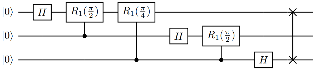
This lower level view of quantum information processing is often described in terms of quantum circuits, which represent the sequential application of gates, or operations, to specific qubits of a system. Thus, the single- and multi-qubit operations you sequentially apply can be readily represented in circuit diagrams. For example, the full three-qubit quantum Fourier transform used in this tutorial has the following representation as a circuit:
Prerequisites
The latest version of Visual Studio Code (VS Code) or open VS Code for the Web.
The latest version of the Microsoft Quantum Development Kit (QDK) extension. For installation details, see Set up the QDK extension.
To use Jupyter Notebooks, install the Python and Jupyter extensions in VS Code.
The latest
qdkPython package with thejupyterextra. To install these, open a terminal and run the following command:pip install --upgrade "qdk[jupyter]"
Create a new Q# file
- In VS Code, open the File menu and choose New Text File.
- Save the file as QFTcircuit.qs. This file contains the Q# code for your program.
- Open QFTcircuit.qs.
Write a QFT circuit in Q#
The first part of this tutorial consists of defining the Q# operation Main, which performs the quantum Fourier transform on three qubits. The DumpMachine function is used to observe how the simulated wavefunction of the three-qubit system evolves across the operation. In the second part of the tutorial, you add measurement functionality and compare the pre- and post-measurement states of the qubits.
You build the operation step by step. Copy and paste the code in the following sections into the QFTcircuit.qs file.
You can view the full Q# code for this section as reference.
Import required Q# libraries
Inside your Q# file, import the relevant Std.* namespaces.
import Std.Diagnostics.*;
import Std.Math.*;
import Std.Arrays.*;

// operations go here
Define operations with arguments and returns
Next, define the Main operation:
operation Main() : Unit {
    // do stuff
}
The Main operation never takes arguments, and for now returns a Unit object, which is analogous to returning void in C# or an empty tuple, Tuple[()], in Python.
Later, you modify the operation to return an array of measurement results.
Allocate qubits
Within the Q# operation, allocate a register of three qubits with the use keyword. With use, the qubits are automatically allocated in the $\ket{0}$ state.
use qs = Qubit[3]; // allocate three qubits

Message("Initial state |000>:");
DumpMachine();
As in real quantum computations, Q# doesn't allow you to directly access qubit states. However, the DumpMachine operation prints the target machine's current state, so it can provide valuable insight for debugging and learning when used together with the full state simulator.
Apply single-qubit and controlled operations
Next, apply the operations that comprise the Main operation itself. Q# already contains many of these, and other basic quantum operations, in the Std.Intrinsic namespace.
Note
Std.Intrinsic wasn't imported in the earlier code snippet with the other namespaces, as it is loaded automatically by the compiler for all Q# programs.
The first operation applied is the H (Hadamard) operation to the first qubit:
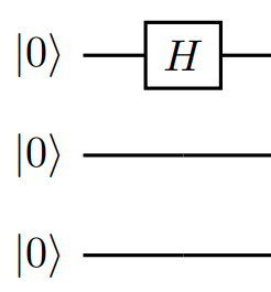
To apply an operation to a specific qubit from a register (for example, a single Qubit from an array Qubit[]), use standard index notation.
So, applying the H operation to the first qubit of the register qs takes the form:
H(qs[0]);
Besides applying the H operation to individual qubits, the QFT circuit consists primarily of controlled R1 rotations. A R1(θ, <qubit>) operation in general leaves the $\ket{0}$ component of the qubit unchanged while applying a rotation of $e^{i\theta}$ to the $\ket{1}$ component.
Q# makes it easy to condition the run of an operation upon one, or multiple, control qubits. In general, the call is prefaced with Controlled, and the operation arguments change as follows:
Op(<normal args>) $\to$ Controlled Op([<control qubits>], (<normal args>))
Note that the control qubit argument must be an array, even if it is for a single qubit.
The controlled operations in the QFT are the R1 operations that act on the first qubit (and controlled by the second and third qubits):
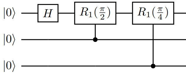
In your Q# file, call these operations with these statements:
Controlled R1([qs[1]], (PI()/2.0, qs[0]));
Controlled R1([qs[2]], (PI()/4.0, qs[0]));
The PI() function is used to define the rotations in terms of pi radians.
Apply SWAP operation
After applying the relevant H operations and controlled rotations to the second and third qubits, the circuit looks like this:
//second qubit:
H(qs[1]);
Controlled R1([qs[2]], (PI()/2.0, qs[1]));

//third qubit:
H(qs[2]);
Finally, you apply a SWAP operation to the first and third qubits to complete the circuit. This operation is necessary because the quantum Fourier transform outputs the qubits in reverse order, so the swaps allow for seamless integration of the subroutine into larger algorithms.
SWAP(qs[2], qs[0]);
The Q# operation now includes the qubit-level operations of the quantum Fourier transform:
Deallocate qubits
The last step is to call DumpMachine() again to see the post-operation state, and to deallocate the qubits. The qubits were in state $\ket{0}$ when you allocated them and need to be reset to their initial state using the ResetAll operation.
Requiring that all qubits be explicitly reset to $\ket{0}$ is a basic feature of Q#, as it allows other operations to know their state precisely when they begin using those same qubits (a scarce resource). Additionally, resetting them assures that they aren't entangled with any other qubits in the system. If the reset isn't performed at the end of a use allocation block, a runtime error might be thrown.
Add the following lines to your Q# file:
Message("After:");
DumpMachine();

ResetAll(qs); // deallocate qubits
The complete QFT operation
The Q# program is complete. Your QFTcircuit.qs file should now look like this:
import Std.Diagnostics.*;
import Std.Math.*;
import Std.Arrays.*;

operation Main() : Unit {

    use qs = Qubit[3]; // allocate three qubits

    Message("Initial state |000>:");
    DumpMachine();

    //QFT:
    //first qubit:
    H(qs[0]);
    Controlled R1([qs[1]], (PI()/2.0, qs[0]));
    Controlled R1([qs[2]], (PI()/4.0, qs[0]));

    //second qubit:
    H(qs[1]);
    Controlled R1([qs[2]], (PI()/2.0, qs[1]));

    //third qubit:
    H(qs[2]);

    SWAP(qs[2], qs[0]);

    Message("After:");
    DumpMachine();

    ResetAll(qs); // deallocate qubits

}
Run the QFT circuit
For now, the Main operation doesn't return any value - the operation returns Unit value. Later, you modify the operation to return an array of measurement results (Result[]).
- To run your program, choose Run Q# File from the menu that precedes
Main, or press Ctrl + F5. The program runs theMainoperation on the default simulator. - The
MessageandDumpMachineoutputs display in the debug console.
If you're curious about how other input states are affected, experiment with applying other qubit operations before the transform.
Add measurements to the QFT circuit
The display from the DumpMachine function showed the results of the operation, but unfortunately, a cornerstone of quantum mechanics states that a real quantum system can't have such a DumpMachine function.
Instead, the information is extracted through measurements, which in general not only fail to provide information on the full quantum state, but can also drastically alter the system itself.
There are many sorts of quantum measurements, but the example here focuses on the most basic: projective measurements on single qubits. Upon measurement in a given basis (for example, the computational basis $ { \ket{0}, \ket{1} } $), the qubit state is projected onto whichever basis state was measured, hence destroying any superposition between the two.
Modify the QFT operation
To implement measurements within a Q# program, use the M operation, which returns a Result type.
First, modify the Main operation to return an array of measurement results, Result[], instead of Unit.
operation Main() : Result[] {
Define and initialize Result[] array
Before allocating qubits, declare and bind a three-element array (one Result for each qubit):
mutable resultArray = [Zero, size = 3];
The mutable keyword prefacing resultArray allows the variable to be modified later in the code, for example, when adding measurement results.
Perform measurements in a for loop and add results to array
After the QFT transform operations, insert the following code:
for i in IndexRange(qs) {
    resultArray w/= i <- M(qs[i]);
}
The IndexRange function called on an array (for example, the array of qubits, qs) returns a range over the indices of the array.
Here, it's used in the for loop to sequentially measure each qubit using the M(qs[i]) statement.
Each measured Result type (either Zero or One) is then added to the corresponding index position in resultArray with an update-and-reassign statement.
Note
The syntax of this statement is unique to Q#, but corresponds to the similar variable reassignment resultArray[i] <- M(qs[i]) seen in other languages such as F# and R.
The keyword set is always used to reassign variables bound using mutable.
Return resultArray
With all three qubits measured and the results added to resultArray, you're safe to reset and deallocate the qubits as before. To
return the measurements, insert:
return resultArray;
Run the QFT circuit with the measurements
Now change the placement of the DumpMachine functions to output the state before and after the measurements.
Your final Q# code should look like this:
import Std.Diagnostics.*;
import Std.Math.*;
import Std.Arrays.*;

operation Main() : Result[] {

    mutable resultArray = [Zero, size = 3];

    use qs = Qubit[3];

    //QFT:
    //first qubit:
    H(qs[0]);
    Controlled R1([qs[1]], (PI()/2.0, qs[0]));
    Controlled R1([qs[2]], (PI()/4.0, qs[0]));

    //second qubit:
    H(qs[1]);
    Controlled R1([qs[2]], (PI()/2.0, qs[1]));

    //third qubit:
    H(qs[2]);

    SWAP(qs[2], qs[0]);

    Message("Before measurement: ");
    DumpMachine();

    for i in IndexRange(qs) {
        resultArray w/= i <- M(qs[i]);
    }

    Message("After measurement: ");
    DumpMachine();

    ResetAll(qs);
    Message("Post-QFT measurement results [qubit0, qubit1, qubit2]: ");
    return resultArray;

}
Tip
Remember to save your file every time you introduce a change to the code before running it again.
- To run your program, choose Run Q# from the menu that precedes
Main, or press Ctrl + F5. The program runs theMainoperation on the default simulator. - The
MessageandDumpMachineoutputs display in the debug console.
Your output should look similar to this:
Before measurement:

 Basis | Amplitude      | Probability | Phase
 -----------------------------------------------
 |000⟩ |  0.3536+0.0000𝑖 |    12.5000% |   0.0000
 |001⟩ |  0.3536+0.0000𝑖 |    12.5000% |   0.0000
 |010⟩ |  0.3536+0.0000𝑖 |    12.5000% |   0.0000
 |011⟩ |  0.3536+0.0000𝑖 |    12.5000% |   0.0000
 |100⟩ |  0.3536+0.0000𝑖 |    12.5000% |   0.0000
 |101⟩ |  0.3536+0.0000𝑖 |    12.5000% |   0.0000
 |110⟩ |  0.3536+0.0000𝑖 |    12.5000% |   0.0000
 |111⟩ |  0.3536+0.0000𝑖 |    12.5000% |   0.0000

After measurement:

 Basis | Amplitude      | Probability | Phase
 -----------------------------------------------
 |010⟩ |  1.0000+0.0000𝑖 |   100.0000% |   0.0000

Post-QFT measurement results [qubit0, qubit1, qubit2]:

[Zero, One, Zero]
This output illustrates a few different things:
- When comparing the returned result to the pre-measurement
DumpMachine, it clearly does not illustrate the post-QFT superposition over basis states. A measurement only returns a single basis state, with a probability determined by the amplitude of that state in the system's wavefunction. - From the post-measurement
DumpMachine, measurement changes the state itself, projecting it from the initial superposition over basis states to the single basis state that corresponds to the measured value.
If you repeat this operation many times, the result statistics begin to illustrate the equally weighted superposition of the post-QFT state that gives rise to a random result on each shot. However, besides being inefficient and still imperfect, this would nevertheless only reproduce the relative amplitudes of the basis states, not the relative phases between them. The latter isn't an issue in this example, but relative phases display if given a more complex input to the QFT than $\ket{000}$.
Use the Q# operations to simplify the QFT circuit
As mentioned in the introduction, much of Q#'s power rests in the fact that it allows you to abstract-away the worries of dealing with individual qubits.
Indeed, if you want to develop full-scale, applicable quantum programs, worrying about whether an H operation goes before or after a particular rotation would only slow you down. Azure Quantum provides the ApplyQFT operation, which you can use and apply for any number of qubits.
Replace everything from the first
Hoperation to theSWAPoperation, inclusive, with:ApplyQFT(qs);Your code should now look like this
import Std.Diagnostics.*;
import Std.Math.*;
import Std.Arrays.*;

operation Main() : Result[] {

    mutable resultArray = [Zero, size = 3];

    use qs = Qubit[3];

    //QFT:
    //first qubit:

    ApplyQFT(qs);

    Message("Before measurement: ");
    DumpMachine();

    for i in IndexRange(qs) {
        resultArray w/= i <- M(qs[i]);
    }

    Message("After measurement: ");
    DumpMachine();

    ResetAll(qs);
    Message("Post-QFT measurement results [qubit0, qubit1, qubit2]: ");
    return resultArray;

}
Run the Q# program again and notice that the output is the same as before.
To see the real benefit of using Q# operations, change the number of qubits to something other than
3:
mutable resultArray = [Zero, size = 4];

use qs = Qubit[4];
//...
You can thus apply the proper QFT for any given number of qubits, without having to worry about adding new H operations and rotations on each qubit.
Related content
Explore other Q# tutorials:
- Quantum random number generator shows how to write a Q# program that generates random numbers out of qubits in superposition.
- Grover's search algorithm shows how to write a Q# program that uses Grover's search algorithm.
- Quantum entanglement shows how to write a Q# program that manipulates and measures qubits and demonstrates the effects of superposition and entanglement.
- The Quantum Katas are self-paced tutorials and programming exercises aimed at teaching the elements of quantum computing and Q# programming at the same time.