Note
Access to this page requires authorization. You can try signing in or changing directories.
Access to this page requires authorization. You can try changing directories.
Important
Support for Machine Learning Studio (classic) will end on 31 August 2024. We recommend you transition to Azure Machine Learning by that date.
Beginning 1 December 2021, you will not be able to create new Machine Learning Studio (classic) resources. Through 31 August 2024, you can continue to use the existing Machine Learning Studio (classic) resources.
- See information on moving machine learning projects from ML Studio (classic) to Azure Machine Learning.
- Learn more about Azure Machine Learning.
ML Studio (classic) documentation is being retired and may not be updated in the future.
Fits a specified probability distribution function to a dataset
Category: Statistical Functions
Note
Applies to: Machine Learning Studio (classic) only
Similar drag-and-drop modules are available in Azure Machine Learning designer.
Module overview
This article describes how to use the Evaluate Probability Function module in Machine Learning Studio (classic), to calculate statistical measures that describe a column’s distribution, such as the Bernoulli, Pareto, or Poisson distributions.
To use this model, connect a dataset that contains at least one column of numerical values, and choose a probability distribution to test. The module returns a data table that contains values from the specified probability function.
You can compute any of these values for the chosen probability distribution:
- cumulative distribution function (cdf)
- inverse cumulative distribution function (InverseCdf)
- probability density function (Pdf)
Why is the probability distribution useful?
When you evaluate your data against a probability distribution, you are mapping column values against a set of values with known properties. By knowing whether your data corresponds to one of these well-known distributions, you might be able infer other properties of your data. In general, you can get better predictions from a model when you can identify the distribution that fits the data best.
The question of which probability distribution function to use depends on the data and the variables that are being measured. For example, some distributions are designed to describe probabilities of discrete values; others are intended for use only with continuous numerical variables. For some distributions, you must also know in advance an expected mean, degrees of freedom, and so forth. For details, see Supported Probability Distributions
How to configure Evaluate Probability Function
All options change depending on the type of probability distribution you want to compute. If you change the probability distribution method, other selections you might have made are reset.
Therefore, be sure to choose the Distribution option first!
The dataset used as input should contains numerical data. Other types of data are ignored.
For each analysis, you can apply a single probability distribution method. To compute a different probability distribution, add a separate instance of the module for each distribution you intend to test.
Add the Evaluate Probability Function module to your experiment. You can find this module in the Statistical Functions category in Machine Learning Studio (classic).
Connect a dataset that contains at least one column of numbers.
Use the Distribution option to select the kind of probability distribution that you want to calculate. See Supported Probability Distributions for a list of options and their required arguments.
Set any parameters that are required by the distribution.
Choose one of three statistics to create: the cumulative distribution function (cdf), inverse cumulative distribution function (InverseCdf), or Probability density function (pdf).
See the Technical notes section for definitions.
Use the column selector to choose the columns over which to compute the selected probability distribution.
All the columns you select must have a numerical data type.
The range of data in the column must also be valid, given the selected probability function. Otherwise, an error or NaN result may occur.
For sparse columns, any values that correspond to background zeros will not be processed.
Use the Result mode option to specify how to output the results. You can replace column values with the probability distribution values, append the new values to the dataset, or return only the probability distribution values.
Run the experiment, or right-click the Evaluate Probability Function module and click Run selected.
Results
The following table contains a example of results, using the Append option, on a single temperature column from the Forest Fires sample dataset.
| temp | StandardNormal.Cdf(temp) | StandardNormal.Pdf(temp) | FFisher.cdf(temp | FFisher.cdf(temp |
|---|---|---|---|---|
| 8.2 | 1 | 1 | 0.984774 | 0.004349 |
| 18 | 1 | 1 | 0.997896 | 0.000311 |
| 14.6 | 1 | 1 | 0.996352 | 0.000648 |
| 8.3 | 1 | 1 | 0.985201 | 0.004187 |
| 11.4 | 1 | 1 | 0.993147 | 0.001502 |
The headings of the generated columns contain the probability distribution that was used.
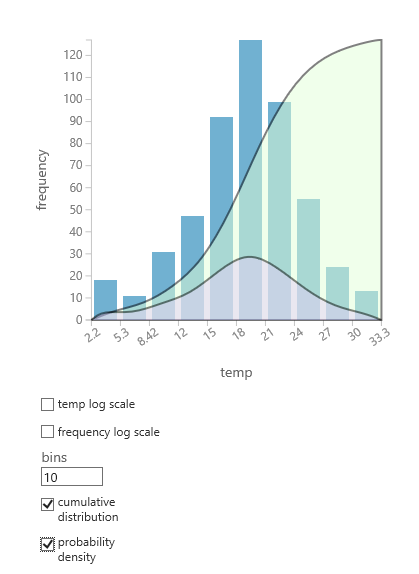
If you are not sure which probability distribution is likely to suit your data, you can create a quick chart of cumulative distribution and probability density for any numeric column.
- Right-click the dataset or module output, and select Visualize.
- Select the column of interest, and in the Histogram pane, select cumulative distribution or probability density.
- A chart of the distribution, like the following, is superimposed on the histogram representing the data.
Supported probability distributions
The Evaluate Probability Function module supports the following distributions:
Bernoulli
The Bernoulli distribution is a distribution over binary values: in other words, it models the expected distribution when only two values are possible.
To calculate, select Bernoulli, and set the following options:
- Probability of success
The parameter p specifies the probability that a 1 is generated. Type a number (float) between 0.0 and 1.0 that specifies the probability of success. The default is .5.
Beta
The Beta distribution is a continuous univariate distribution.
To calculate, select Beta, and set the following options:
Shape
Type a value to change the shape of the distribution.A shape parameter is any parameter of a probability distribution that does not define its location or scale. Therefore, when you enter a value for shape, the parameter changes the shape of the distribution rather than moving, stretching, or shrinking it.
The value must be a number (
double). The default is 1.0.Scale
Type a number to use for scaling the distribution.By applying a scale value to the distribution, you can shrink or stretch it.
The default value is 1.0. Values must be positive numbers.
Upper bound
Type a number (double) that represents the upper bound of the distribution. The default is 1.0.Lower bound
Type a number (double) that represents the lower bound of the distribution. The default is 0.0.
Binomial
The binomial distribution is a discrete univariate distribution. The binomial distribution is used to model the number of successes in a sample. Replacement is used when sampling. For sampling without replacement, use the Hypergeometric distribution.
To calculate, select Binomial, and set the following options:
Probability of success
Type a number (float) between 0.0 and 1.0 that indicates the probability of success. The default is .5.Number of trials
Specify the number of trials.Use an
integer, with a minimum value of 1. The default is 3.
Cauchy
The Cauchy distribution is a symmetric continuous probability distribution.
To calculate, select Cauchy, and set the following options:
Location
Type a number (double) that represents the location of the 0th element.By specifying a value for the Location parameter, you can shift the probability distribution up or down a numeric scale.
The default is 0.0.
ChiSquare
The chi-square distribution is a sum of the squares of k independent, standard, normal, random variables.
To calculate, select ChiSquare, and set the following options:
- Number of degrees of freedom
Type a number (
double) to specify the degrees of freedom. The default is 1.0.
ChiSquareRightTailed
This option provides a right-tailed chi-squared distribution.
To calculate, select ChiSquareRightTailed, and set the following options:
- Number of degrees of freedom
Type a number (double) to specify the degrees of freedom. The default is 1.0.
Exponential
The exponential distribution is a distribution over the real numbers parameterized by one non-negative parameter.
To calculate, select Exponential, and set the following options:
- Lambda
Type a number (double) to use as the lambda parameter. The default is 1.0.
FFisher
Generates the probability of the Fisher statistic for a sample, also known as the Fisher F-distribution. This distribution is two-tailed.
To calculate, select FFisher, and set the following options:
Numerator degrees of freedom
Type a number (double) to specify the degrees of freedom that is used in the numerator. The default is 3.0.Denominator degrees of freedom
Type a number (double) to specify the degrees of freedom that is used in the denominator. The default is 6.0.
FFisherRightTailed
Creates a right-tailed Fisher distribution. The Fisher distribution is also known as the Fisher F-distribution, Snedecor distribution, or Fisher-Snedecor distribution. This particular form of the distribution is right-tailed.
To calculate, select FFisherRightTailed, and set the following options:
Numerator degrees of freedom
Type a number (double) to specify the degrees of freedom that is used in the numerator. The default is 3.0.Denominator degrees of freedom
Type a number (double) to specify the degrees of freedom that is used in the denominator. The default is 6.0.
Gamma
The gamma distribution is a family of continuous probability distributions with two parameters. For example, chi-squared is a special case of the gamma distribution.
To calculate, select Gamma, and set the following options:
Scale
Type a value to use for scaling the distribution.By applying a scale value to the distribution, you can shrink or stretch it.
The default value is 1.0. Values must be positive numbers.
Location
Type a number (double) that represents the location of the 0th element.By specifying a value for the Location parameter, you can shift the probability distribution up or down a numeric scale.
The default is 0.0.
GeneralizedExtremeValues
Creates a distribution developed to handle extreme values. The generalized extreme value (GEV) distribution is actually a group of continuous probability distributions that combines the Gumbel, Fréchet, and Weibull distributions (also known as type I, II, and III extreme value distributions).
For more information about extreme value theory, see this article in Wikipedia: Fisher-Tippet-Gnedenko theorem.
To calculate, select GeneralizedExtremeValues, and set the following options:
Shape
Type a value to change the shape of the distribution.A shape parameter is any parameter of a probability distribution that does not define its location or scale. Therefore, when you enter a value for shape, the parameter changes the shape of the distribution rather than moving, stretching, or shrinking it.
The value must be a number (
double). The default is 1.0.Scale
Type a value to use for scaling the distribution.By applying a scale value to the distribution, you can shrink or stretch it.
The default value is 1.0. Values must be positive numbers.
Location
Type a number (double) that represents the location of the 0th element.By typing a value for the Location parameter, you can shift the probability distribution up or down a numeric scale.
The default is 0.0.
Geometric
The geometric distribution is a distribution over positive integers parameterized by one positive real number.
To calculate, select Geometric, and set the following options:
- Probability of success
Type a number (float) between 0.0 and 1.0 that indicates the probability of success. The default is .5.
Note
This implementation of the geometric distribution does not generate zeros.
GumbelMax
The Gumbel distribution is one of several extreme value distributions. The GumbelMax option implements the Maximum Extreme Value Type 1 distribution.
To calculate, select GumbelMax, and set the following options:
Scale
Type a value to use for scaling the distribution.By applying a scale value to the distribution, you can shrink or stretch it.
The default value is 1.0. Values must be positive numbers.
Location
Type a number (double) that represents the location of the 0th element.By typing a value for the Location parameter, you can shift the probability distribution up or down a numeric scale.
The default is 0.0.
GumbelMin
The Gumbel distribution is one of several extreme value distributions. The Gumbel distribution is also referred to as the Smallest Extreme Value (SEV) distribution or the Smallest Extreme Value (Type I) distribution. The GumbelMin option implements the Minimum Extreme Value Type 1 distribution.
To calculate, select GumbelMin, and must set the following options:
Scale
Type a value to use for scaling the distribution.By applying a scale value to the distribution, you can shrink or stretch it.
The default value is 1.0. Values must be positive numbers.
Location
Type a number (double) that represents the location of the 0th element.By typing a value for the Location parameter, you can shift the probability distribution up or down a numeric scale.
The default is 0.0.
Hypergeometric
The hypergeometric distribution is a discrete probability distribution that describes the number of successes in a sequence of n draws from a finite population without replacement, just as the binomial distribution describes the number of successes for draws with replacement.
To calculate, select Hypergeometric, and set the following options:
Number of samples
Type an integer that indicates the number of samples to use. The default is 9.Number of success
Type an integer that defines the value for success. The default is 24.Population size
Specify the population size to use when estimating the hypergeometric distribution.
Laplace
The Laplace distribution is a distribution over the real numbers, parameterized by a mean and by a scale parameter.
To calculate, select Laplace distribution, and set the following options:
Scale
Type a value to use for scaling the distribution.By applying a scale value to the distribution, you can shrink or stretch it.
The default value is 1.0. Values must be positive numbers.
Location
Type a number (double) that represents the location of the 0th element.By typing a value for the Location parameter, you can shift the probability distribution up or down a numeric scale.
The default is 0.0.
Logistic
The logistic distribution is similar to the normal distribution, but it has no limit on the left side of the distribution. The logistic distribution is used in logistic regression and neural network models and for modeling life sciences data.
To calculate, select Logistic, and set the following options:
Scale
Type a value to use for scaling the distribution.By applying a scale value to the distribution, you can shrink or stretch it.
The default value is 1.0. Values must be positive numbers.
Mean
Type a number (double)that indicates the estimated mean value of the distribution. The default is 0.0.
Lognormal
The lognormal distribution is a continuous univariate distribution.
To calculate, select Lognormal, and set the following options:
Mean
Type a number (double) that indicates the estimated mean value of the distribution. The default is 0.0.Standard deviation
Type a positive number (double) that indicates the estimated standard deviation of the distribution. The default is 1.0.
NegativeBinomial
The negative binomial distribution is a distribution over the natural numbers with two parameters (r, p). In the special case that r is an integer, you can interpret the distribution as the number of tails before the rth head when the probability of the head is p.
To calculate, select NegativeBinomial, and set the following options:
Probability of success
Type a number (float) between 0.0 and 1.0 that indicates the probability of success. The default is .5.Number of success
Type an integer that specifies the value for success. The default is 24.
Normal
The normal distribution is also known as the Gaussian distribution.
To calculate, select Normal, and set the following options:
Mean
Type a number (double) that indicates the estimated mean value of the distribution. The default is 0.0.Standard deviation
Type a positive number (double) that indicates the estimated standard deviation of the distribution. The default is 1.0.
Pareto
The Pareto distribution is a power-law probability distribution that coincides with social, scientific, geophysical, actuarial, and many other types of observable phenomena.
To calculate, select Pareto, and set the following options:
Shape
Type a value (optional) to change the shape of the distribution.A shape parameter is any parameter of a probability distribution that does not define its location or scale. Therefore, when you enter a value for shape, the parameter changes the shape of the distribution rather than moving, stretching, or shrinking it.
The value must be a number (
double). The default is 1.0.Scale
Type a value (optional) to change the scale of the distribution. By applying a scale value to the distribution, you can shrink or stretch it.The value must be a number (
double). The default is 1.0.
Poisson
In this implementation, Knuth's method is used to generate Poisson distributed random variables. For more information about the Poisson distribution, see Poisson Regression.
To calculate, select Poisson, and set the following options:
- Mean
Type a number (double) that indicates the estimated mean value of the distribution. The default is 0.0.
Rayleigh
The Rayleigh distribution is a continuous probability distribution. As an example of how it arises, the wind speed will have a Rayleigh distribution if the components of the two-dimensional wind velocity vector are uncorrelated and normally distributed with equal variance.
To calculate, select Rayleigh, and set the following options:
- Lower bound
Type a number (double) that represents the lower bound of the distribution. The default is 0.0.
StandardNormal
This option provides the standard normal distribution, with no other parameters.
To calculate, select StandardNormal, and select the columns.
TStudent
This option implements the univariate Student’s t-distribution.
To calculate, select TStudent, and set the following options:
- Number of degrees of freedom
Type a number (double) to specify the degrees of freedom. The default is 1.0.
TStudentRightTailed
Implements the univariate Student’s t-distribution by using one right tail.
To calculate, select TStudentRightTailed, and set the following options:
- Number of degrees of freedom
Type a number (double) to specify the degrees of freedom. The default is 1.0.
TStudentTwoTailed
Implements a two-tailed Student’s t-distribution.
To calculate, select TStudentTwoTailed, and set the following options:
- Number of degrees of freedom
Type a number (double) to specify the degrees of freedom. The default is 1.0.
Uniform
The uniform distribution is also known as the rectangular distribution.
To calculate, select Uniform, and set the following options:
Lower bound
Type a number (double) that represents the lower limit of the distribution. The default is 0.0.Upper bound
Type a number (double) that represents the upper limit of the distribution. The default is 1.0.
Weibull
The Weibull distribution is widely used in reliability engineering. You can use its Shape parameter to model many other distributions.
To calculate, select Weibull, and set the following options:
Shape
Type a value (optional) to change the shape of the distribution.A shape parameter is any parameter of a probability distribution that does not define its location or scale. Therefore, when you enter a value for shape, the parameter changes the shape of the distribution rather than moving, stretching, or shrinking it.
The value must be a number (
double). The default is 1.0.Scale
Type a value (optional) to change the scale of the distribution. By applying a scale value to the distribution, you can shrink or stretch it.The value must be a number (
double). The default is 1.0.
Technical notes
This section contains implementation details, tips, and answers to frequently asked questions.
Implementation details
This module supports all distributions that are provided in the open source MATH.NET Numerics library. For more information, see the documentation for the Math.Net.Numerics.Distribution library.
Right-tailed and two-tailed distributions appear as separate distributions, not as parameterized versions of base distributions. The current behavior is to preserve compatibility with Excel.
Definitions
This module supports calculating any of these values for the specified distribution:
cdf, or the cumulative distribution function
Returns the probability for a compound event, defined as the sum of ocurrences when the random variable takes a value smaller than some specific value x.
In other words, it answers the question: "How common are samples that are less than or equal to this value?"
This function can be used with both continuous and discrete numeric variables.
InverseCdf, or the inverse cumulative distribution function
Returns the value associated with a specific cumulative probability value (cdf).
In other words, it answers the question: "What is the value of x at which the cdf function returns the cumulative probability y?"
pdf, or the probability density function
Describes the relative likelihood for a random variable to be a specific value.
In other words, it answers the question: "How common are samples at exactly this value?"
Expected inputs
| Name | Type | Description |
|---|---|---|
| Dataset | Data Table | Input dataset |
Module parameters
| Name | Range | Type | Default | Description |
|---|---|---|---|---|
| Distribution | Any | ProbabilityDistribution | StandardNormal | Select the kind of probability distribution to generate. |
| Method | Any | ProbabilityDistributionMethod | Cdf | Select the method to use when calculating the selected probability distribution. Options are the cumulative distribution function (cdf), the inverse cumulative distribution function (InverseCdf), and the probability density function or mass function (pdf). |
| Negative binomial distribution method | Any | ProbabilityDistributionMethodForNegativeBinomial | Cdf | If you select the negative binomial distribution, specify the method used for evaluating the distribution. |
| Probability of success | [0.0;1.0] | Float | 0.5 | Type a value to use as the probability of success. |
| Shape | Any | Float | 1.0 | Type a value that modifies the shape of the distribution. |
| Scale | >=0.0 | Float | 1.0 | Type a value that changes the scale of the distribution to expand or shrink it in size. |
| Number of trials | >=1 | Integer | 3 | Specify the number of trials. |
| Lower bound | Any | Float | 0.0 | Type a number to use as the lower limit of the distribution |
| Upper bound | Any | Float | 1.0 | Type a number to use as the upper limit of the distribution |
| Location | Any | Float | 0.0 | Type the location of the zero element in the distribution. |
| Number of degrees of freedom | Any | Float | 1.0 | Specify the number of degrees of freedom. |
| Numerator degrees of freedom | Any | Float | 3.0 | Specify the number of degrees of freedom in the numerator. |
| Denominator degrees of freedom | Any | Float | 6.0 | Specify the number of degrees of freedom in the denominator. |
| Lambda | >=0.0 | Float | 1.0 | Specify a value for the Lambda parameter. |
| Number of samples | Any | Integer | 9 | Specify the number of samples. |
| Number of success | Any | Integer | 24 | Type a value to use as the number of success. |
| Population size | Any | Integer | 52 | Specify the population size. |
| Mean | Any | Float | 0.0 | Type the estimated mean value. |
| Standard deviation | >=0.0 | Float | 1.0 | Type the estimated standard deviation. |
| Column set | Any | ColumnSelection | Choose the columns over which to calculate the probability distribution. | |
| Result mode | Any | OutputTo | ResultOnly | Specify how the results are to be saved in the output dataset. The options are to append new columns, replace existing columns, or output only the results. |
Output
| Name | Type | Description |
|---|---|---|
| Results dataset | Data Table | Output dataset |
Exception
For a complete list of error messages, see Module Error Codes.
| Exception | Description |
|---|---|
| Error 0017 | Exception occurs if one or more specified columns have a type that is unsupported by the current module. |
For a list of errors specific to Studio (classic) modules, see Machine Learning Error codes.
For a list of API exceptions, see Machine Learning REST API Error Codes.