Overview
 |
Terrain and Scenery
The terrain system in ESP consists of eight main data components, elevation (DEM data), imagery, land classification, water classification, regions, seasons, population density, and vector data. All sets of data can be replaced in whole or in part by new data, perhaps providing a higher resolution, or sometimes simply alternative data. The main tasks that are covered by this document are:
- The Terrain System: An overview of how the seven terrain components work together.
- The tools used to modify or replace the default data.
See Also
Table of Contents
- The Terrain System
- Regions
- Land Classification
- Elevations
- Seasons
- Water Classification
- Population Density
- Base File Information
- The Shp2Vec Tool
- The TmfViewer Tool
- The Resample Tool
- Resample Samples
- Appendix I: The World Coordinate System
- Appendix II: The Naming Convention for Terrain Textures
The Terrain System
The terrain system is optimized to minimize disk space. Whereas it would be technically possible to create the entire world from satellite imagery and high resolution elevation data, this would involve an enormous amount of data and is still not a practicable proposition, even with the huge storage space available on DVDs. Because of this, it is possible to improve on terrain and scenery in specific local areas. Before going into how to make these improvements in detail, this section describes how the system functions by default.
The key to the terrain system is a grid, where the World is divided into squares, roughly 1.2km on each side. Using this concept, information is held on the World for the following properties: geographical region, population density, land classification, water classification and season. For example, if an aircraft is flying over one of these grid squares in North America, this information can be used not only to build a good approximation of the terrain, but also provide information on how busy the highways are likely to be. At exactly the same simulated time, an aircraft flying in the southern hemisphere may well be flying in a different season, and even though the land classification may be identical to the grid square in North America, the rendering of that land can be different because of regional variations in what trees make up a forest, or shrub is present on a desert, for example. The grid system is not used for actual terrain imagery or elevations, but as reference information so that the correct textures can be located for any area.
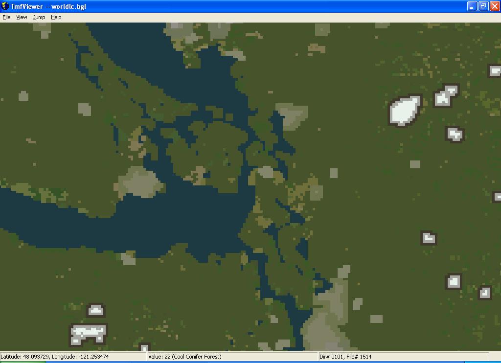
The following image shows the land classification for the southern tip of Vancouver Island, Seattle, and some of the Cascade mountains. The 1.2km squares are very evident in the data. To view the default data, run the TmfViewer.exe tool. Using this tool you can examine the BGL files that contain the default grid data.
 |
Regions
The following diagram shows the geographical regions the world is divided into.
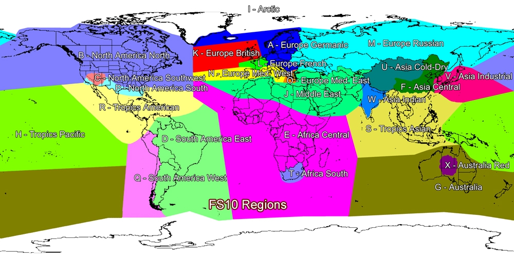 |
The regions are:
- A: Europe Germanic
- B: North America North
- C: North America Southwest
- D: South America East
- E: Africa Central
- F: Asia Central
- G: Australia
- H: Tropics Pacific
- I: Arctic
- J: Middle East
- K: Europe British
- L: Europe French
- M: Europe Russian
- N: Europe Mediterranean West
- O: Europe Mediterranean East
- P: North America South
- Q: South America West
- R: Tropics American
- S: Tropics Asian
- T: Africa South
- U: Asia Cold-Dry
- V: Asia Industrial
- W: Asia Indian
- X: Australia Red
Note that Antarctica and the interior of Iceland are classified as Artic, but the coastline of Iceland falls into the Europe Germanic category.
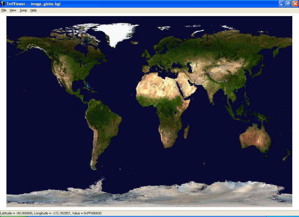
Using TmfViewer first load in the image of the world -- stored in the Microsoft ESP\1.0\Scenery\World\Scenery folder. This can be used as a background image with other information appearing as overlays.
 |
Next, from the Microsoft ESP\1.0\Scenery\Base\Scenery folder, load in the regions.bgl file. This will show the regions overlaid onto the world map, as follows:
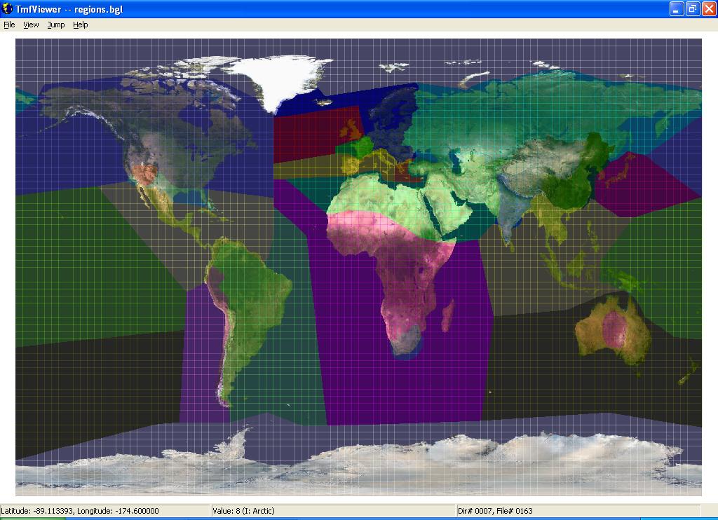 |
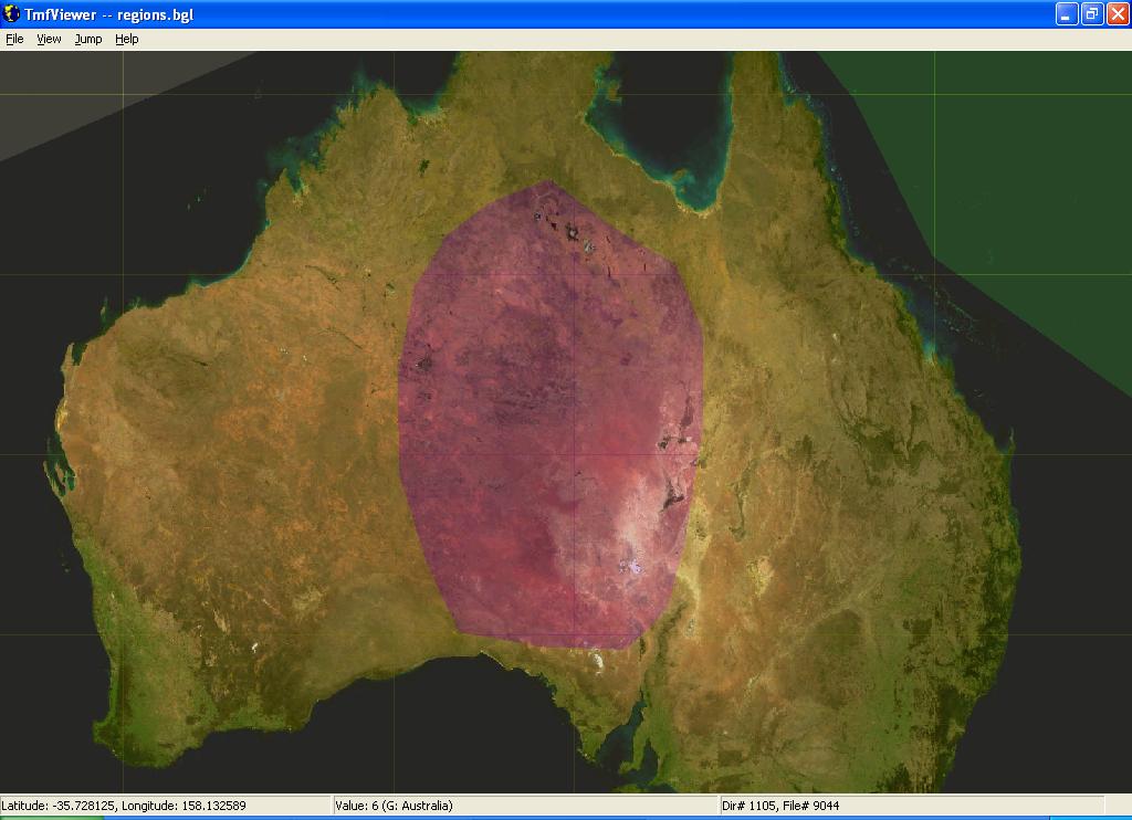
To zoom in on a particular area of the world, first just click the mouse on the area of interest, then press the Numpad + key to zoom in (or Numpad - to zoom out). For example, to examine the center of Australia in more detail, click on the red region in the center, then press Numpad + a few times, and you should get the following image:
 |
It is possible to change the regions that have been applied to the world, though it is not possible to add new regions to the 24 listed above.
Land Classification
Next load up TmfViewer again, this time with just the worldlc.bgl file, in the Microsoft ESP\1.0\Scenery\Base\Scenery folder. This contains all the land classification data.
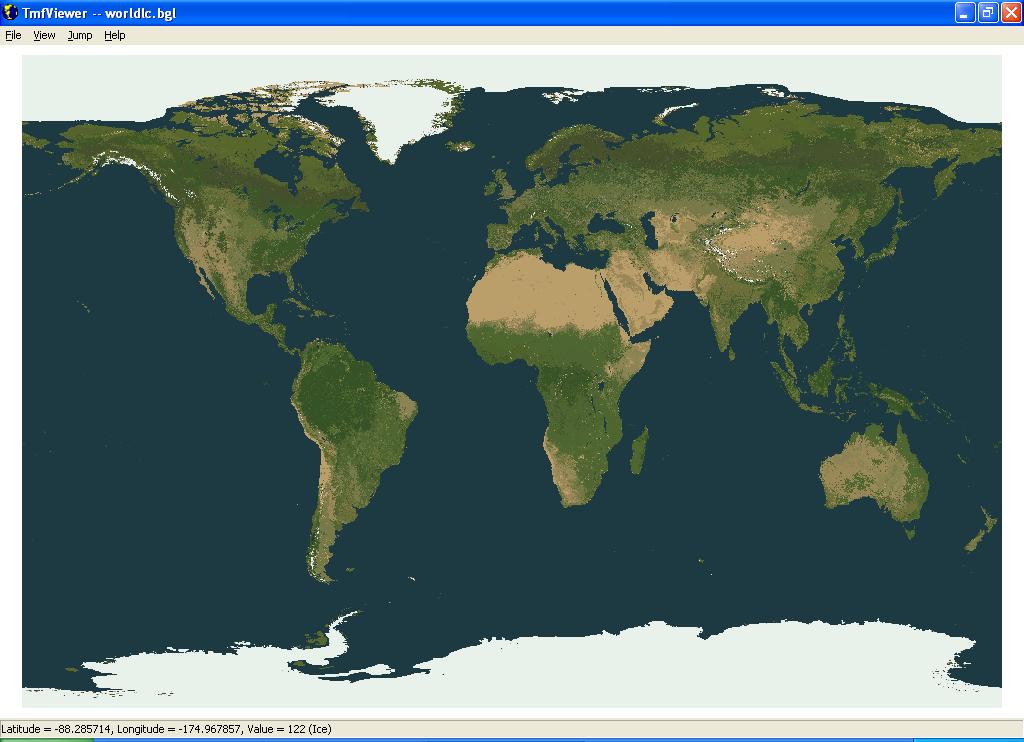 |
Each color coded square in the grid corresponds with a single land type from the Olson Land Classification Table, shown below. It is not possible to provide a greater degree of resolution than the 1.2km squares of the grid, it is possible to change the land classification to a different value from the table.
Olson Land Classification Table
For any square on the land classification grid, a single value from the following table applies.
| 0 | Ocean, Sea, Large Lake |
| 1 | Large City Urban Grid Wet |
| 2 | Low Sparse Grassland |
| 3 | Coniferous Forest |
| 4 | Deciduous Conifer Forest |
| 5 | Deciduous Broadleaf Forest |
| 6 | Evergreen Broadleaf Forests |
| 7 | Tall Grasses And Shrubs |
| 8 | Bare Desert |
| 9 | Upland Tundra |
| 10 | Irrigated Grassland |
| 11 | Semi Desert |
| 12 | Dry Crop and Town |
| 13 | Wooded Wet Swamp |
| 14 | ### Unused ### |
| 15 | ### Unused ### |
| 16 | Shrub Evergreen |
| 17 | Shrub Deciduous |
| 18 | ### Unused ### |
| 19 | Evergreen Forest And Fields |
| 20 | Cool Rain Forest |
| 21 | Conifer Boreal Forest |
| 22 | Cool Conifer Forest |
| 23 | Cool Mixed Forest |
| 24 | Mixed Forest |
| 25 | Cool Broadleaf Forest |
| 26 | Southern Deciduous Broadleaf Forest |
| 27 | Conifer Forest |
| 28 | Montane Tropical Forests |
| 29 | Seasonal Tropical Forest |
| 30 | Cool Crops And Towns |
| 31 | Crops And Town |
| 32 | Dry Tropical Woods |
| 33 | Tropical Rainforest |
| 34 | Tropical Degraded Forest |
| 35 | Corn And Beans Cropland |
| 36 | Rice Paddy And Field |
| 37 | Hot Irrigated Cropland |
| 38 | Cool Irrigated Cropland |
| 39 | ### Unused ### |
| 40 | Cool Grasses And Shrubs |
| 41 | Hot And Mild Grasses And Shrubs |
| 42 | Cold Grassland |
| 43 | Savanna (Woods) |
| 44 | Mire Bog Fen |
| 45 | Marsh Wetland |
| 46 | Mediterranean Scrub |
| 47 | Dry Woody Scrub |
| 48 | Dry Evergreen Woods |
| 49 | ### Unused ### |
| 50 | Sand Desert |
| 51 | Semi Desert Shrubs |
| 52 | Semi Desert Sage |
| 53 | Barren Tundra |
| 54 | Cool Southern Hemisphere Mixed Forests |
| 55 | Cool Fields And Woods |
| 56 | Forest And Field |
| 57 | Cool Forest And Field |
| 58 | Fields And Woody Savanna |
| 59 | Succulent And Thorn Scrub |
| 60 | Small Leaf Mixed Woods |
| 61 | Deciduous And Mixed Boreal Forest |
| 62 | Narrow Conifers |
| 63 | Wooded Tundra |
| 64 | Heath Scrub |
| 65 | ### Unused ### |
| 66 | ### Unused ### |
| 67 | ### Unused ### |
| 68 | ### Unused ### |
| 69 | Polar And Alpine Desert |
| 70 | ### Unused ### |
| 71 | ### Unused ### |
| 72 | Mangrove |
| 73 | ### Unused ### |
| 74 | ### Unused ### |
| 75 | ### Unused ### |
| 76 | Crop And Water Mixtures |
| 77 | ### Unused ### |
| 78 | Southern Hemisphere Mixed Forest |
| 79 | ### Unused ### |
| 80 | ### Unused ### |
| 81 | ### Unused ### |
| 82 | ### Unused ### |
| 83 | ### Unused ### |
| 84 | ### Unused ### |
| 85 | ### Unused ### |
| 86 | ### Unused ### |
| 87 | ### Unused ### |
| 88 | ### Unused ### |
| 89 | Moist Eucalyptus |
| 90 | Rain Green Tropical Forest |
| 91 | Woody Savanna |
| 92 | Broadleaf Crops |
| 93 | Grass Crops |
| 94 | Crops Grass Shrubs |
| 95 | Grass Skirting 1 |
| 96 | Grass Skirting 2 |
| 97 | Grass and Shrub Skirting |
| 98 | Dry Grass and Dirt Skirting |
| 99 | Sand and Desert Skirting |
| 100 | Ocean, Sea, Large Lake |
| 101 | Large City Urban Grid Wet |
| 102 | Large City Urban Grid Dry |
| 103 | Large City Urban Non Grid Wet |
| 104 | Large City Urban Non Grid Dry |
| 105 | Medium City Urban Grid Wet |
| 106 | Medium City Urban Grid Dry |
| 107 | Medium City Urban Non Grid Wet |
| 108 | Medium City Urban Non Grid Dry |
| 109 | Large City Suburban Grid Wet |
| 110 | Large City Suburban Grid Dry |
| 111 | Large City Suburban Non Grid Wet |
| 112 | Large City Suburban Non Grid Dry |
| 113 | Medium City Suburban Grid Wet |
| 114 | Medium City Suburban Grid Dry |
| 115 | Medium City Suburban Non Grid Wet |
| 116 | Medium City Suburban Non Grid Dry |
| 117 | Small City Suburban Grid Wet |
| 118 | Small City Suburban Grid Dry |
| 119 | Small City Suburban Non Grid Wet |
| 120 | Small City Suburban Non Grid Dry |
| 121 | Large City High-rise |
| 122 | Ice |
| 123 | Inland Water |
| 124 | Ocean Inlet |
| 125 | Non Perennial Inland Water |
| 126 | Non Perennial Inland Sea |
| 127 | Reef |
| 128 | Grass |
| 129 | Arid |
| 130 | Rock |
| 131 | Dirt |
| 132 | Coral |
| 133 | Lava |
| 134 | Park |
| 135 | Golf Course |
| 136 | Cement |
| 137 | Tan Sand Beach |
| 138 | Black Sand Beach |
| 139 | Airfield1 |
| 140 | Airfield2 |
| 141 | Rock Volcanic |
| 142 | Rock Ice |
| 143 | Glacier Ice |
| 144 | Evergreen Tree Crop |
| 145 | Deciduous Tree Crop |
| 146 | Desert Rock |
| 147 | Savanna Grass |
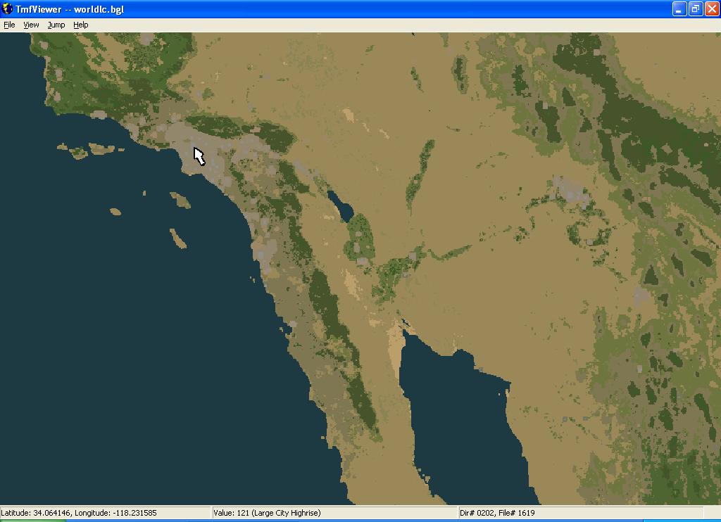
Use TmfViewer to zoom in on the area around San Diego. Notice that if you place the mouse over any grid square the Olson class value is given, along with the latitude and longitude, for that square. Although classifications are color coded within the tool, this method of placing the mouse and reading the value is the most precise way of determining land class values.
 |
Elevations
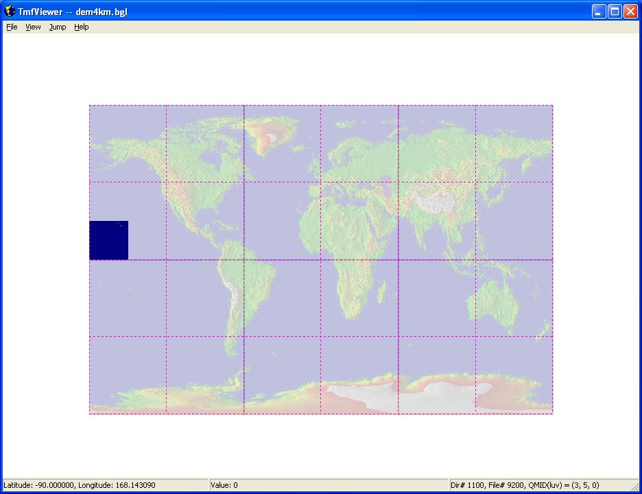
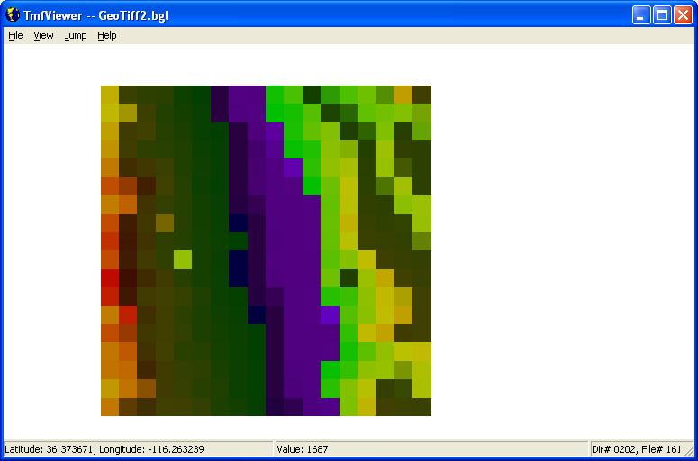
To draw the landscape, elevation data is held in the dem4km.bgl file, also in the Microsoft ESP\1.0\Scenery\Base\Scenery folder. See the section on Base File Information for details on where this elevation data is stored. And compare the lower and higher resolution elevation data for Hawaii below.
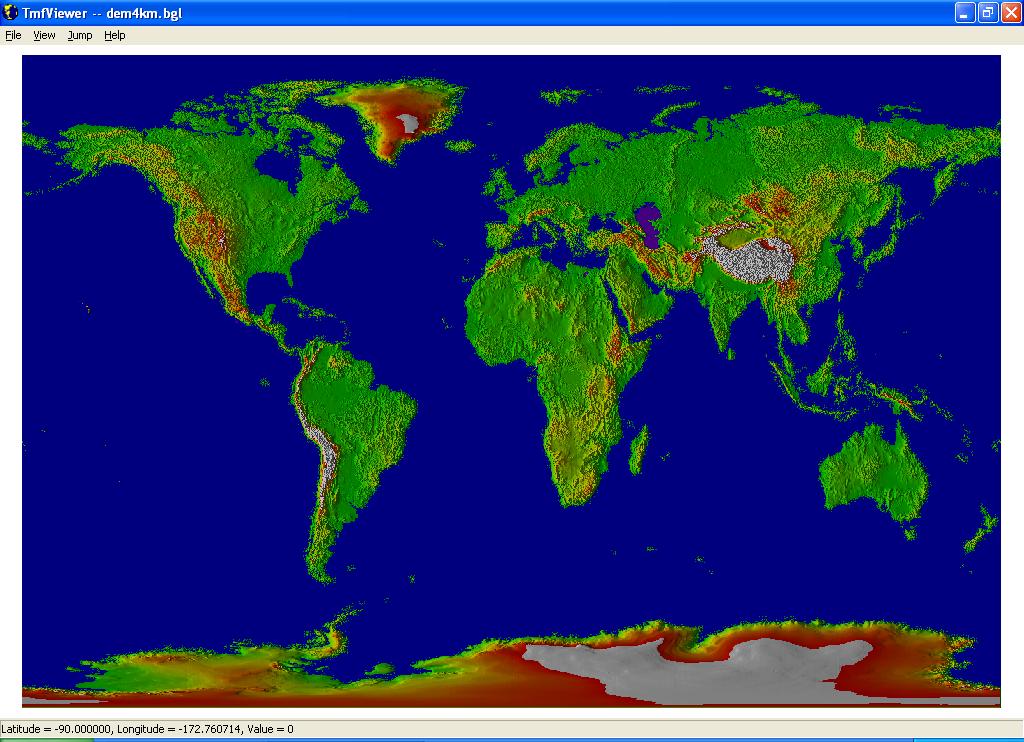 |
The following image shows the old elevation data for Hawaii, note the value given in the information bar is 3904. This is the height in meters of the square the mouse is pointing at.
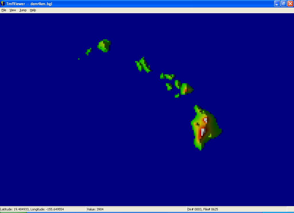 |
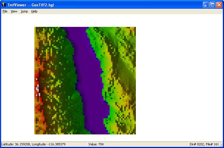
The higher resolution elevation data for Hawaii provides the following image.
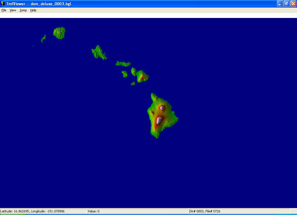 |
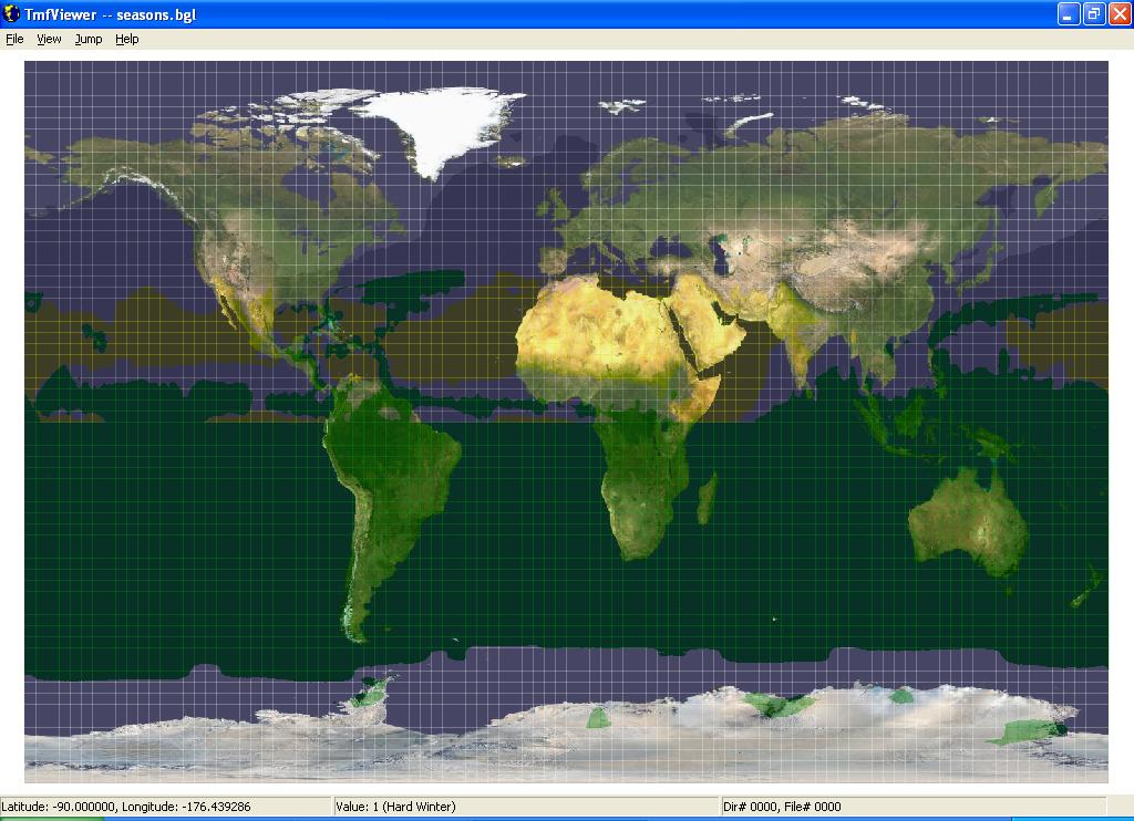
Seasons
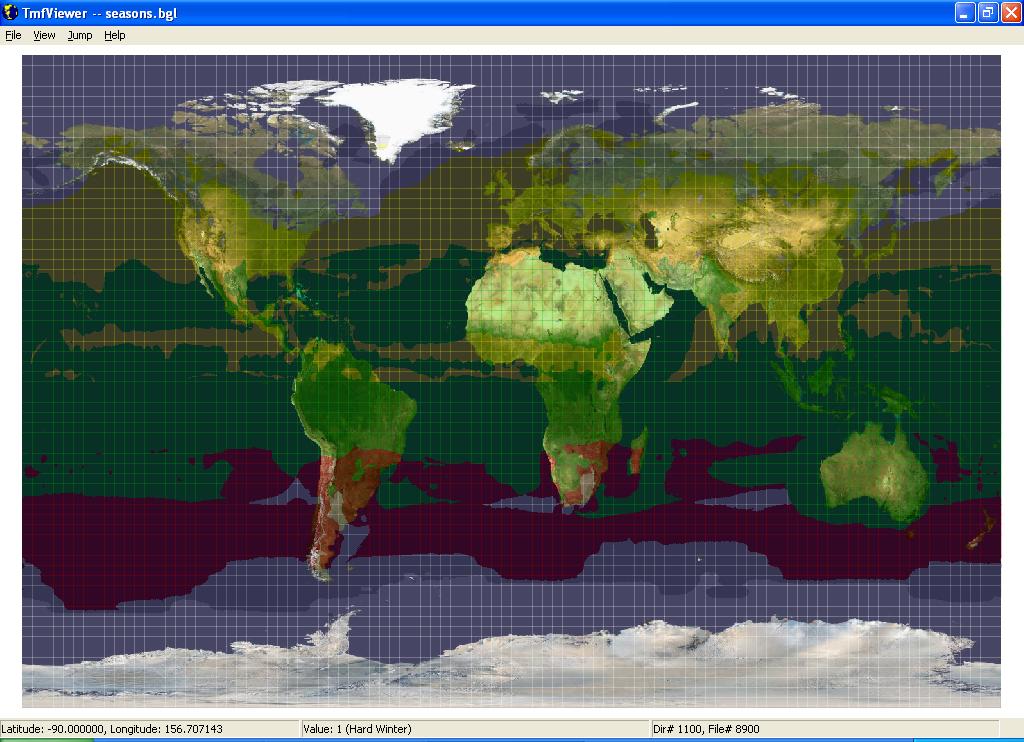
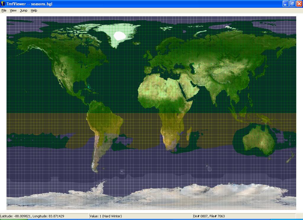
There are five seasons: Spring (SP), Summer (SU), Fall (FA), Winter (WI), and Hard Winter (HW). The main difference between the two winter textures, WI and HW, is the snow on the ground in Hard Winter. Seasons are different across the world at any one time, and this information is held by ESP for the 12 months of the year. Seasonal information does not vary at all in the simulation within a month, and changes on midnight at the end of the month to the new season. The following table shows the season information for four months of the year. Note that green identifies summer, yellow is spring, red is fall, grey is mild winter, and white is hard winter.
 |
 |
 |
|
To view the season information using TmfViewer, first load up the image_globe.bgl file from Microsoft ESP\1.0\Scenery\World\Scenery. Note that the first image loaded into this tool is always opaque. The next images loaded can be drawn transparent, so the outline of the countries/regions and continents shows through.
Next load up the seasons.bgl file from Microsoft ESP\1.0\Scenery\Base\Scenery. Use the View menu to select the various months of the year.
Water Classification
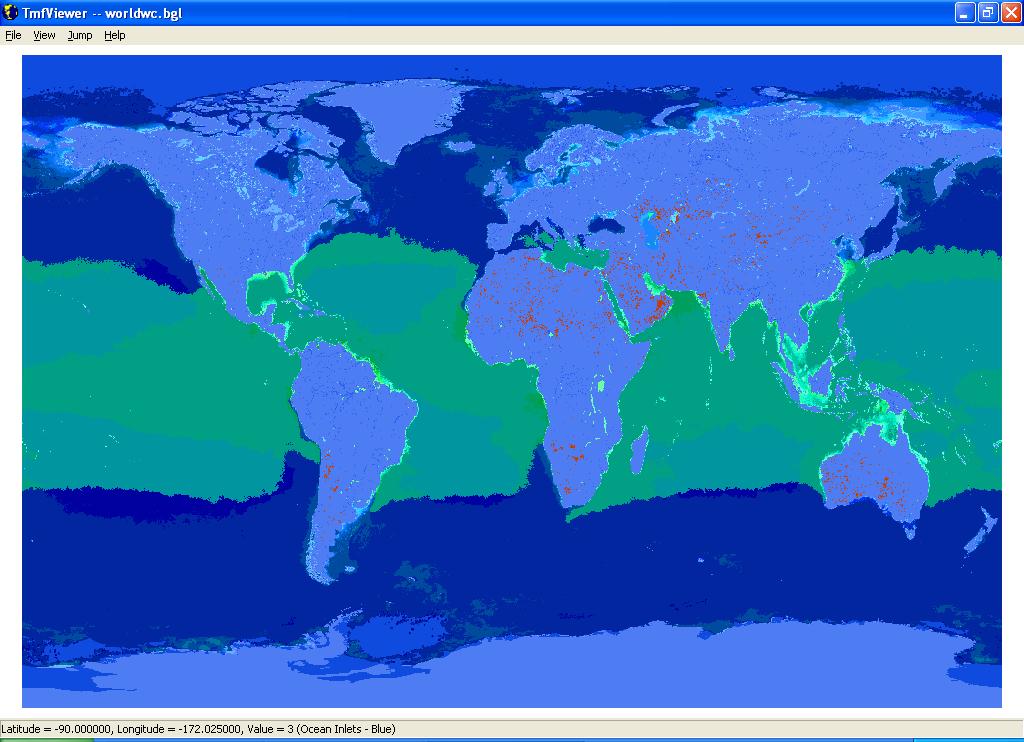
There is not the same broad range of types and variants present in the water classes that are found in the land textures. By default, water classes use one region and have one season, one variation, and no night texture. To give greater visual control, water is categorized by depth, plankton concentration, and whether it is tropical. The depth tends to dictate the darkness of the water color: the deeper the water, the darker the texture. The plankton concentration determines the amount of green in the water color: the more plankton, the greener the water. Tropical waters are highlighted because they tend to have a more vibrant color. Load up worldwc.bgl to see the water classification map:
 |
The following definitions are used for water depth:
- Shallow Ocean Water 1: 0-5m
- Shallow Ocean Water 2: 6-15m
- Shallow Ocean Water 3: 16-30m
- Shallow Ocean Water 4: 31-50m
- Medium Depth Ocean Water: 51-80m
- Deep Ocean Water: >80m
The following table shows the colors used for the water classes in TmfViewer, and the classification numbers and descriptions. Note that the color used in TmfViewer does not match the actual color of the water when rendered in the simulation, but in most cases is a close approximation.
| 1- Shallow Inland Water - Blue 2 - Deep Inland Water - Blue 3 - Ocean Inlets - Blue 4 - Non Perennial Inland Sea - Blue 5 - Non Perennial Inland Water - Blue 6 - Outflow Water - Blue 7- Shallow Inland Water - Brown 8 - Deep Inland Water - Brown 9 - Ocean Inlets - Brown 10 - Non Perennial Inland Sea - Brown 11 - Non Perennial Inland Water - Brown 12- Outflow Water - Brown 13 - Shallow Ocean Water 1 - Class1 (High Plankton Concentration) 14 - Shallow Ocean Water 2 - Class1 (High Plankton Concentration) 15 - Shallow Ocean Water 3 - Class1 (High Plankton Concentration) 16 - Shallow Ocean Water 4 - Class1 (High Plankton Concentration) 17 - Medium Depth Ocean Water - Class1 (High Plankton Concentration) 18 - Deep Ocean Water - Class1 (High Plankton Concentration) 19 - Shallow Ocean Water 1 - Class2 ( Med High Plankton Concentration) 20 - Shallow Ocean Water 2 - Class2 ( Med High Plankton Concentration) 21 - Shallow Ocean Water 3 - Class2 ( Med High Plankton Concentration) 22 - Shallow Ocean Water 4 - Class2 ( Med High Plankton Concentration) 23 - Medium Depth Ocean Water - Class2 ( Med High Plankton Concentration) 24 - Deep Ocean Water - Class2 (Med High Plankton Concentration) 25 - Shallow Ocean Water 1 - Class3 (Med Low Plankton Concentration) 26 - Shallow Ocean Water 2 - Class3 (Med Low Plankton Concentration) 27 - Shallow Ocean Water 3 - Class3 (Med Low Plankton Concentration) 28 - Shallow Ocean Water 4 - Class3 (Med Low Plankton Concentration) 29 - Medium Depth Ocean Water - Class3 (Med Low Plankton Concentration) 30 - Deep Ocean Water - Class3 (Med Low Plankton Concentration) 31 - Shallow Ocean Water 1 - Class4 (Low Plankton Concentration) 32 - Shallow Ocean Water 2 - Class4 (Low Plankton Concentration) 33 - Shallow Ocean Water 3 - Class4 (Low Plankton Concentration) 34 - Shallow Ocean Water 4 - Class4 (Low Plankton Concentration) 35 - Medium Depth Ocean Water - Class4 (Low Plankton Concentration) 36 - Deep Ocean Water - Class4 (Low Plankton Concentration) 37 - Shallow Ocean Water 1 - Class1 (High Plankton Concentration), Tropical 38 - Shallow Ocean Water 2 - Class1 (High Plankton Concentration), Tropical 39 - Shallow Ocean Water 3 - Class1 (High Plankton Concentration), Tropical 40 - Shallow Ocean Water 4 - Class1 (High Plankton Concentration),Tropical 41 - Medium Depth Ocean Water - Class1 (High Plankton Concentration), Tropical 42 - Deep Ocean Water - Class1 (High Plankton Concentration), Tropical 43 - Shallow Ocean Water 1 - Class2 ( Med High Plankton Concentration), Tropical 44 - Shallow Ocean Water 2 - Class2 ( Med High Plankton Concentration), Tropical 45 - Shallow Ocean Water 3 - Class2 ( Med High Plankton Concentration), Tropical 46 - Shallow Ocean Water 4 - Class2 ( Med High Plankton Concentration), Tropical 47 - Medium Depth Ocean Water - Class2 ( Med High Plankton Concentration), Tropical 48 - Deep Ocean Water - Class2 (Med High Plankton Concentration), Tropical 49 - Shallow Ocean Water 1 - Class3 (Med Low Plankton Concentration), Tropical 50 - Shallow Ocean Water 2 - Class3 (Med Low Plankton Concentration), Tropical 51 - Shallow Ocean Water 3 - Class3 (Med Low Plankton Concentration), Tropical 52 - Shallow Ocean Water 4 - Class3 (Med Low Plankton Concentration), Tropical 53 - Medium Depth Ocean Water - Class3 (Med Low Plankton Concentration), Tropical 54 - Deep Ocean Water - Class3 (Med Low Plankton Concentration), Tropical 55 - Shallow Ocean Water 1 - Class4 (Low Plankton Concentration), Tropical 56 - Shallow Ocean Water 2 - Class4 (Low Plankton Concentration), Tropical 57 - Shallow Ocean Water 3 - Class4 (Low Plankton Concentration), Tropical 58 - Shallow Ocean Water 4 - Class4 (Low Plankton Concentration), Tropical 59 - Medium Depth Ocean Water - Class4 (Low Plankton Concentration), Tropical 60- Deep Ocean Water - Class4 (Low Plankton Concentration), Tropical |
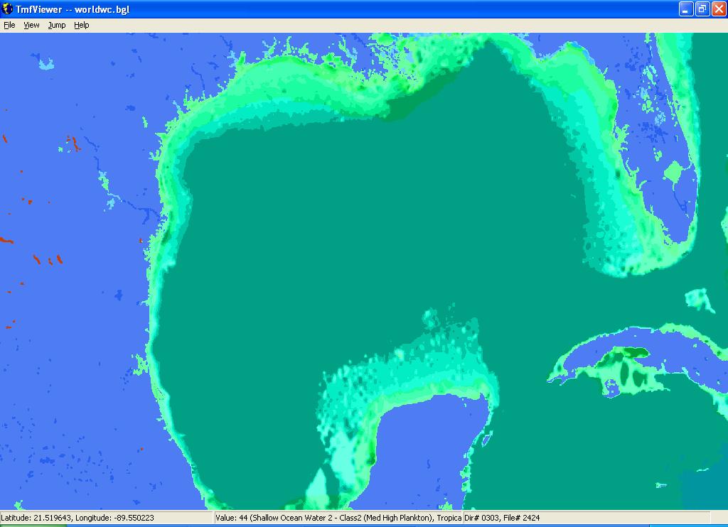
The following image shows a close up of the Gulf of Mexico, the light green areas clearly denoting the Shallow Inland Water classifications.
 |
Population Density
The population density of an area helps provide some guidelines as to the amount of traffic that is on the highways, recreational boat traffic on lakes, train frequency, and so on. Population density is held in values from 0 (no people) to 100 (very high density city). Note that black, used to identify the zero population case, occurs in several land locations in the map below.
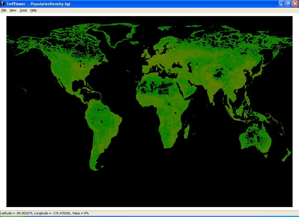 |
The following image shows the population density map for some of the northeast coast of the United States. The very high concentrations around the cities of Boston, New York and Philadelphia are very evident.
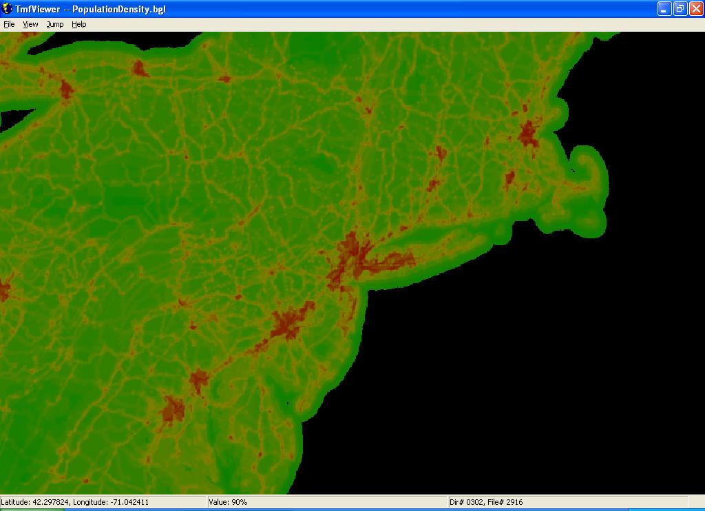 |
Base File Information
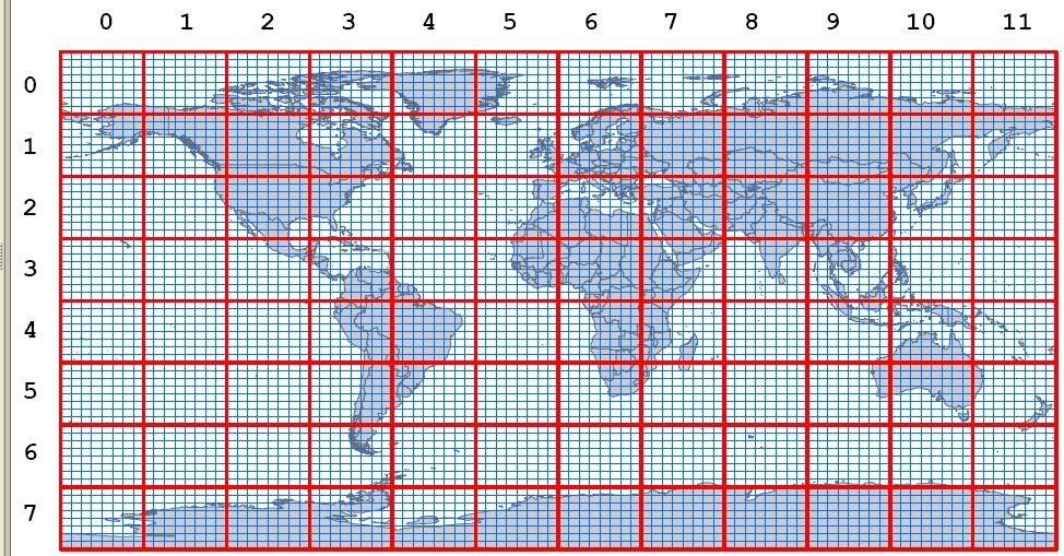
The file system used to store all the terrain information is based around the following grid. In Microsoft ESP\1.0\Scenery you will notice many folders with numeric names such as 0000, 1107, and so on. The first two numbers refer to the column of data (from 00 to 11) and the second two to the row of data (from 00 to 07). So 0000 contains the default information for the top left hand rectangle in the diagram below, and 1107 the information for the bottom right hand rectangle. Each of the larger rectangles (shown in red) is divided into smaller rectangles (shown in blue).
There are 8 x 8 smaller rectangles within each larger one. These smaller rectangles reference scenery and vector data that is present within that area. These are also numbered column first, then row, so the small grid square 7824, for example, is the area around Hong Kong SAR (which falls in the large grid square 0903). This is a different grid system than the 1.2Km squares used previously. This system is used to organize the data files in a reasonably logical way. The large grid squares represent QMID level 4, the smaller squares QMID level 7 (see QMID and LOD values for more details).
 |
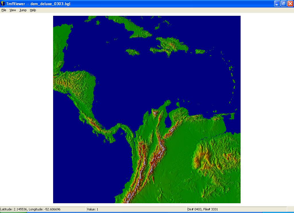
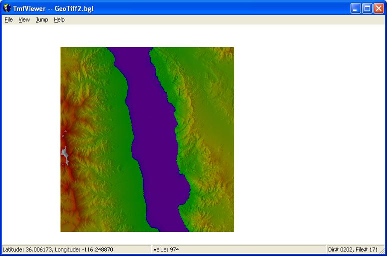
If you take, for example, the folder 0303, this will contain data for much of the Caribbean Sea. Use TmfViewer to open the dem0303.bgl file in this folder, and you will see the following high resolution elevation data image. Each of the numbered directories will contain elevation data with demNNNN in the filename. This higher resolution data is used to draw the landscape accurately when using ESP. See the Elevations section for a comparison of lower and higher resolution images of Hawaii.
 |
TmfViewer can also be used to examine the vector data (roads, rivers, streams and so on) for an area of the above grid. For example, open the file cvx7824.bgl (in the folder scenery/0903/scenery). Use the + key to zoom in and you will see the following vector data applies to the area around Hong Kong SAR. Clearly the red lines are major highways, the blue lines are streams, the grey lines are utilities, the yellow areas are airport boundaries and the green areas are parks. Right click near a vector to be given the option Identify Vector Features, which can be used to give details on the type of the vector.
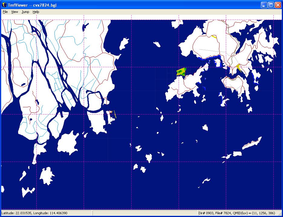 |
The Shp2Vec Tool
The Shp2Vec (shape file to vector data) tool is in the SDK\Environment Kit\Terrain SDK folder. This tool takes vector shape data and creates the BGL files used by ESP. The vector shape data is in standard ESRI shape file format. This format includes three file types, .shp (shape data), shx (shape index data), and .dbf (database file containing attributes of the shape data). The ESRI shapefile is a public domain format for the interchange of GIS (geographical information system) data. The wide availability of tools which support the shapefile format and the fact that the format is publicly documented made it the logical choice as the input to the Shp2Vec tool.
The Shp2Vec tool is command line driven, and takes the following parameters:
>Shp2Vec path string -flags
The path points to the folder containing all the shape data. Use a single period to specify the current folder. All shape files in the specified folder, but not any sub-folder, are examined by the tool if the filename contains the string as part of the filename. The first three characters of a file can be anything, but all the remaining characters, except the extension, must be identical to the string. As a convention, the first three characters are set to FLX for airport boundaries, HPX for hydro polygons, and so on (see the table below for a full list), and then the common string is set to the quad numbers. The quad numbers can be located in the Base File Information grid (for example, Hong Kong SAR is in the quad 78 24). The Shp2Vec tool then simply looks for files with the quad string present in the name. For example, if you look at the filenames in the SDK\Environment Kit\Terrain SDK\Vector Examples\Example1\SourceData folder you will see that they all have 7824 as the common string. This means that entering the following line will process all the shape files:
>Shp2Vec Vector Examples\Example1\SourceData 7824
Of course, other file naming conventions could be used. The default behavior of the tool is to provide replacement data for the quad cell. The flag -ADDTOCELLS is optional, and simply indicates the new data should be merged with existing data, and not replace it.
Performing a task with the Shp2Vec tool, such as replacing vector data, or perhaps using surfaces to exclude autogen or land classifications, or to flatten an area to use as an airport boundary, the following general process should be followed:
- Use a shape file editor to create the vector data, or surface shapes, that are the basis of the change. A shape file editor is not provided as part of the SDK. There should be one flavor of data per shapefile. Whereas most vector types only require 2D co-ordinates, ensure that vector data for AirportBounds and WaterPolys is 3D (that is, includes elevation data).
- Create a single folder with the shapefiles in it, named according to a convention but fitting the format described above. Each shapefile consists of a .dbf, a .shx, and a .shp file.
- Add to the folder one of the proprietary XML files supplied with the SDK for each flavor of data. These XML files provide information to the tool. It is very important to point out that they should not be edited, the GUIDs and values in them are hard-coded in ESP, and there is no value in altering the content of these files. However, it is important to rename them within the folder to match the naming of the shape files. So for example, the XML file FLX7824.XML is named to match the airport boundary data of Hong Kong SAR airport contained in the FLX7824 shapefile.
- The .dbf file can be edited, usually in a spreadsheet such as Microsoft Excel®. Usually these edits take the form of replacing GUIDs to match the task you wish to complete. Notice that the columns of the .dbf file exactly match the data definitions in the XML file.
- Run the Shp2Vec giving your folder as input.
The table below links to typical XML files, which are all used in Shp2Vec Example 1, except the exclusions vector data, which is used in Shp2Vec Example 2.
| Airport Boundaries | FLX7824 | Although this area is titled Airport Boundaries, these are used for a number of purposes, including flattening a surface and excluding certain types of data, in addition to defining airport boundaries. The .dbf file contains two columns, UUID and GUID. Enter the following GUIDs in the GUID column to achieve flattening, or Autogen or land class exclusions. Airport boundaries are one example of the use of Flatten + MaskClassMap + ExcludeAutogen. {6c0c6528-5cf1-483a-a586-2c905cf2757e} ExcludeAutogen {47d48287-3ade-4fc5-8bec-b6b36901e612} Flatten {5a7f944c-3d79-4e0c-82f5-04844e5dc653} Flatten + MaskClassMap {1f2baab1-4132-416e-8f6f-28abe79cd60b} MaskClassMap {46bfb3bd-ce68-418e-8112-feba17428ace} Flatten + MaskClassMap + ExcludeAutogen {18580a63-fc8f-4a02-a622-8a1e073e627b} Flatten + ExcludeAutogen {594e70c8-06a5-4e3f-be6e-4dbf50b49d11} MaskClassMap + ExcludeAutogen |
| Hydro Polygons | HPX7824 | These are used for slopes and medium/high resolution water polygons. |
| Streams | STX7824 | This does not include rivers. Rivers are created with polygons matching the terrain. |
| GPS Hydro Polygons | HGX7824 | These are used for low resolution water polygons, and only by GPS systems. |
| Roads | RDX7824 | This provides the graphic and data for the road surface. To have moving traffic appear on the road, a corresponding Freeways entry must be made. There is a significant performance cost in rendering moving road traffic. |
| Freeways | FWX7824 | This indicates moving traffic is drawn. There is no rendered road surface associated with this type, this just defines the path of traffic. Note that where freeways merge into a smaller number of lanes, the traffic on the dropped lanes simply disappears. |
| Utilities | UTX7824 | Includes power lines, telephone lines, and similar data. |
| Shorelines | HLX7824 | Shorelines in this context are those where a breaking wave (surf) effect should appear. Shoreline vectors are directional polylines that must go clockwise around the water polygons. |
| Railways | RRX7824 | These define railways. Currently trains are not featured in ESP, so there is no associated railway traffic entry. |
| Parks | PKX7824 | Although these are named Parks, they are used much more generally as landclass polygons. |
| Exclusions | EXXVHHX | Exclusions are polygons that exclude other shapes whose bounding boxes overlap the bounding box of the exclusion polygon. The use of bounding boxes is less precise than using the actual shape geometry, but it's much faster at run time. Exclusions only apply to shapes that are in lower priority scenery layers in scenery.cfg. You cannot exclude shapes in the same or higher priority scenery layers. These exclusions only apply to vector data, they do not apply to objects created by Autogen (for this, refer to the Airport Boundaries entry). The .dbf file for exclusion polygons have a GUID column, and there are three options for what to enter here: 1. Exclude all vector data by using a null GUID (all zeros). 2. Exclude general classes of features that have an attribute block (for example, all roads or all water polygons) by using one of the GUIDs from the Vector Attributes table. Note that some of the entries affect vector autogen associated with the excluded feature. 3. Exclude specific types of shapes (for example, only one lane gravel roads or only golf course polygons) by using one of the GUIDs listed in Vector Shape Properties GUIDs. |
Notes
- The Shp2Vec tool does not process vector data that crosses 180 degrees Latitude, or the Poles.
- The clip levels are the defaults used by ESP data. Clip level 11 is QMID level 11. Setting higher clip levels will create more detailed data, but at the expense of size and performance. Note the use of clip level 15 for freeways.
Vector Attributes
The following table gives the GUIDs that apply for each type of vector data. Refer to the example XML files on how they are used.
| AirportBounds | 11 | This requires 3D vertices, otherwise this entry will cut deep holes in the landscape. Note there is no special attribute to indicate this requirement. | AirportBounds | {359C73E8-06BE-4FB2-ABCB-EC942F7761D0} | |
| AirportBounds | Guid | 11 | Guid of texture (as text) | Texture | {1B6A15BB-05FB-4401-A8D1-BB520E84904C} |
| AirportBounds | Uuid | 11 | Unique ID (does not go into the simulation) | AirportBounds | {359C73E8-06BE-4FB2-ABCB-EC942F7761D0} |
| Exclusions | Guid | 11 | Guid of texture (as text) | Texture | {1B6A15BB-05FB-4401-A8D1-BB520E84904C} |
| Exclusions | Uuid | 11 | Unique ID (does not go into the simulation) | Exclusions | {AC39CDCB-DB78-4628-9A7C-051DA7AC864A} |
| FreewayTrafficRoads | NumberOfLa | 15 | Note the dbf file format truncates the Output Column type to 10 characters. The number of lanes can be in the range 1 to 9. Guid of texture (as text) | FreewayTrafficRoads | {54B91ED8-BC02-41B7-8C3B-2B8449FF85EC} |
| FreewayTrafficRoads | TrafficDir | 15 | The direction of the traffic is specified in the shape file: F = traffic moves from reference node (one direction, cars drive away from vertex 0 towards vertex N). T = traffic moves towards reference node. Note that the entry B ( both directions ) is not implemented. |
FreewayTrafficRoads | {54B91ED8-BC02-41B7-8C3B-2B8449FF85EC} |
| FreewayTrafficRoads | Uuid | 15 | Unique ID (does not go into the simulation) | FreewayTrafficRoads | {54B91ED8-BC02-41B7-8C3B-2B8449FF85EC} |
| Parks | Guid | 11 | Guid of texture (as text) | Texture | {1B6A15BB-05FB-4401-A8D1-BB520E84904C} |
| Parks | Uuid | 11 | Unique ID (does not go into the simulation) | Parks | {91CB4A9B-9398-48E6-81DA-70AEA3295914} |
| Railways | Guid | 11 | Guid of texture (as text) | Texture | {1B6A15BB-05FB-4401-A8D1-BB520E84904C} |
| Railways | Uuid | 11 | Unique ID (does not go into the simulation) | Railways | {33239EB4-D2B8-46F5-98AB-47B3D0922E2A} |
| Roads | Guid | 11 | Guid of texture (as text) | Texture | {1B6A15BB-05FB-4401-A8D1-BB520E84904C} |
| Roads | Uuid | 11 | Unique ID (does not go into the simulation) | Roads | {560FA8E6-723D-407D-B730-AE08039102A5} |
| Shorelines | Guid | 11 | Guid of texture (as text) | Texture | {1B6A15BB-05FB-4401-A8D1-BB520E84904C} |
| Shorelines | Uuid | 11 | Unique ID (does not go into the simulation) | Shorelines | {0CBC8FAD-DF73-40A1-AD2B-FE62F8004F6F} |
| Streams | Guid | 11 | Guid of texture (as text) | Texture | {1B6A15BB-05FB-4401-A8D1-BB520E84904C} |
| Streams | Uuid | 11 | Unique ID (does not go into the simulation) | Streams | {714BF912-F9DF-467E-80AE-28EB27374DBD} |
| Utilities | Guid | 11 | Guid of texture (as text) | Texture | {1B6A15BB-05FB-4401-A8D1-BB520E84904C} |
| Utilities | Uuid | 11 | Unique ID (does not go into the simulation) | Utilities | {C7ACE4AE-871D-4938-8BDC-BB29C4BBF4E3} |
| WaterPolys | 11 | This requires 3D vertices, otherwise this entry will cut deep holes in the landscape. Note there is no special attribute to indicate this requirement. | WaterPolys | {956A42AD-EC8A-41BE-B7CB-C68B5FF1727E} | |
| WaterPolys | Guid | 11 | Guid of texture (as text) | Texture | {1B6A15BB-05FB-4401-A8D1-BB520E84904C} |
| WaterPolys | SlopeX | 11 | Slope in vertical meters per degree of longitude. 13 char floating point number. | Slope | {CEB07D86-3605-44BE-B48A-97F8D01B74DE} |
| WaterPolys | SlopeY | 11 | Slope in vertical meters per degree of latitude. 13 char floating point number. | Slope | {CEB07D86-3605-44BE-B48A-97F8D01B74DE} |
| WaterPolys | Uuid | 11 | Unique ID (does not go into the simulation) | WaterPolys | {956A42AD-EC8A-41BE-B7CB-C68B5FF1727E} |
| WaterPolysGPS | Uuid | 11 | Unique ID (does not go into the simulation) | WaterPolysGPS | {EA0C44F7-01DE-4D10-97EB-FB5510EB7B72} |
Notes
- The unique IDs that are marked as "does not go into the simulation", are used to troubleshoot issues with the data creation process.
- The texture GUIDs (noted in the Attribute Block column) reference into in the Scenery Configuration File.
Shp2Vec Sample 1: Hong Kong SAR Area
The Vector Examples/Example1/SourceData folder includes all the files for all the types of vector data present around Hong Kong SAR. To run the sample type the following in the command line, after navigating to the SDK\Environment Kit\Terrain SDK folder.
>shp2vec "Vector Examples\Example1\SourceData" 7824
The BGL file will be written to the same folder as the data, an example of the output is in the Vector Examples/Example1/Output folder. The command-line output will give some statistics when the tool runs correctly, for example the output from running the tool with the above example data is shown below:
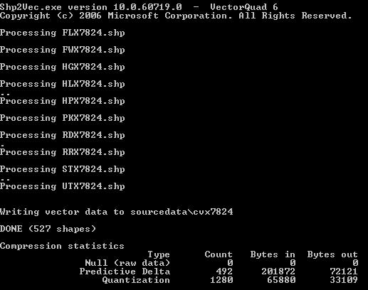 |
Shp2Vec Sample 2: Excluding and Replacing around Hong Kong SAR (VHHH).
The Vector Examples/Example2/SourceData folder includes a sample excluding and then replacing AirportBounds geometry around Hong Kong SAR. To run the sample type the following in the command line, after navigating to the SDK\Environment Kit\Terrain SDK folder.
>shp2vec "Vector Examples\Example2\SourceData" VHHH -ADDTOCELLS
Note the importance of the -ADDTOCELLS flag to add this data to the existing vector data. In the TmfViewer tool, the new airport boundary is shown in the following image.
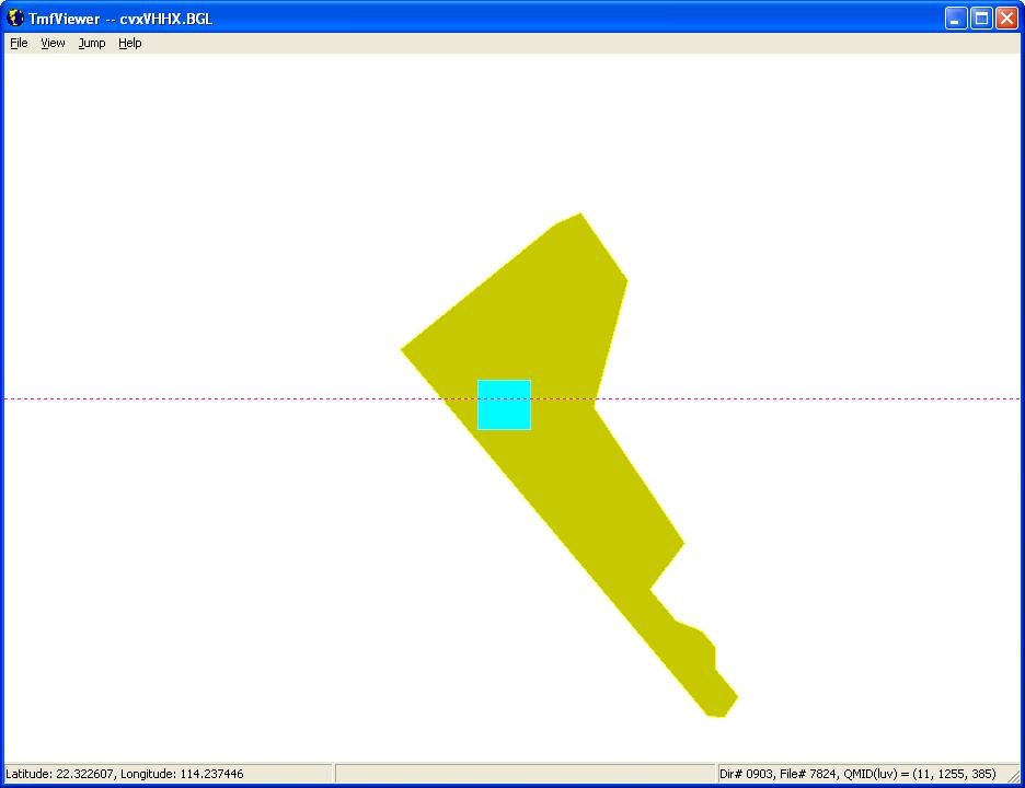 |
The TmfViewer Tool
The TmfViewer tool is in the SDK\Environment Kit\Terrain SDK folder. It can be used to examine many different types of data stored in BGL files. You cannot use this tool to examine all BGL files, however, just those using the World grid system.
Use the File/Open menu item to load a file. Use the Jump menu items to save and use selected map locations. The following table describes the View menu elements of the TmfViewer tool.
| Level of Detail | All the available levels of detail (LOD) contained in the BGL file will be enabled. If an image is loaded and nothing appears, it can be that the Level of Detail is not set to a value that is applicable. Refer to QMID and LOD values for more details. |
| LOD Grid | Draws a grid showing the sizes of the LOD cells. Refer to QMID and LOD values for more details. |
| QMID Grid | Draws a grid showing the sizes of the QMID cells. Refer to QMID and LOD values for more details. |
| Seasons/Variations | If seasonal data is relevant for the BGL file, then the months of the year, and the Night item will be enabled if they are present. |
| Show Missing Data Mask | Selecting this will highlight any areas of data that are missing (that match the NullValue value, refer to the Source Parameters for .inf files more details) with a blue/gray shading. |
| Show Water Mask | Water on a land texture is determined by the alpha channel. Selecting this item will display such areas in blue. |
| Highlight Values ... | This enables all areas with the same data value to be highlighted. For example, if Land Classification data is being examined, and the Land Class highlight value is set to 16 (see the Olson Land Classification table), then all the Shrub Evergreen areas will be highlighted (in bright purple). Highlighting can also be done by right-clicking on an area. All other areas with the same data value will be highlighted. |
| Clear All Highlights | Simply resets all the Highlight Values to -1 (no highlights). |
| Elevation Color Ramp... | The elevation colors are fixed: magenta (lowest elevation), violet, blue, green, yellow, red,, white (highest). Changing the color ramp values changes at what elevation the colors change. |
| Overlay transparency... | The first file loaded by this tool is always drawn opaque. Select this item if subsequent files loaded should be drawn transparent, so the first file shows through. This can be useful when comparing world elevation data, with the world population density, for example. |
| Vector Data | Vector Data is linear data such as roads, streams, utility lines, shorelines, and other similar features. When vector data is loaded into this tool, select which data items that should be displayed. |
| Zoom | Zoom in and out. This can also be done with the Numpad + and Numpad - keys. |
| Pan | Pan North, South, East and West. This can also be done with the up, down, right and left arrow keys. |
The Resample Tool
The key process in replacing or modifying the default data is known as resampling, and the key tool for this process is the resample.exe tool. This is a command line driven tool that takes information from a text file (a .inf file) and then processes the files referenced according to the parameters set. The following section describes the parameters that can be set in an .inf file, and this is followed by a number of worked examples.
The following are the four basic steps required to replace default data.
- Acquire raw digital data (see the Resample Samples for some suggestions).
- Create an .inf file for the raw data.
- Run Resample.exe on the raw data to create a .bgl file.
- Place the new files in the right folders for ESP.
The resample tool is in the SDK\Environment Kit\Terrain SDK folder. The simplest way to use it is to drag a single .inf file onto the Resample tool icon. This is equivalent to a call in the command line: Resample file.inf. Running Resample tool from the command line allows a few options and the use of multiple .inf files, with the following format:
Resample [-i, -q, ?] file1.INF[file2.INF…fileN.INF]
- -i ignores all but the last [Destination] section.
- -q runs in quiet mode.
- ? prints a help message.
All .inf files are text files with at least two sections:
- [Source] provides information on what source file to use, and how to interpret it.
- [Destination] provides information on where the resulting files should be placed.
By default, the resampler scans each .inf file, collecting information from each [Source] section it encounters. Once a [Destination] section is found, it proceeds with the resampling process. If more [Source] sections are thereafter encountered, they are treated as a separate task and these sections will be used when the next [Destination] section is encountered. If the -i switch is specified, resample ignores all but the last [Destination] section, so considers the whole file as a single task.
Multiple .inf files are allowed because it is possible for the [Source] and [Destination] sections to be in separate files. This is convenient when you want to generate different resolutions of data from a single source file. Build an .inf file for the source data and multiple .inf files with [Destination] sections for each destination file. To generate one destination file from multiple source files, create an .inf file with a [Source] section for each file and a .inf file with a [Destination] section and list them all on the command line with the destination .inf file listed last.
Comments
To add a comment to an .inf file, either a whole line or information at the end of a line, add a semi-colon, this indicates to the Resample tool that any text following the semi-colon on the same line be ignored.
Source Parameters
If the file contains multiple source files, then the following section needs to be added to the top of the file (it has an identical [Source] directive to the parameters for a single file). All parameters are of the form Parameter = Value. There can be spaces or tabs either side of the equals sign.
[Source] section
It is possible to define more than one source image in a single .inf file. This is extremely useful when working with imagery that has seasonal and night time variations. To define multiple source images, set the value of the [Source] Type directive to MultiSource. Then add a NumberOfSource directive whose value is the number of source images you want to define. Finally, add additional sections with names like [Source1], [Source2], and so on that contain the source directives for each of the individual source images.
| Type = Multisource | This directive simply informs the resample tool that this is a multi-source file. |
| NumberOfSources =n | The number of [Source] sections in the file. |
[Source] section
The parameters can be listed in any order in the section.
| Type | BMP | Windows bitmap | required | required | required | required | required | |
| TGA | Targa image file | |||||||
| GeoTIFF | GeoTIFF file | |||||||
| TIFF | For TIFF imagery that does not have GeoTIFF georeferencing tags | |||||||
| Raw | Raw BIP, BIL, or BSQ file | |||||||
| SDE | Remote SDE Geodatabase | |||||||
| VectorGDB | Vector data in file or geodatabase | |||||||
| Layer | Elevation Imagery LandClass PopulationDensity Region Season WaterClass None | Elevation data Aerial imagery Land classification data Population density Cultural/environmental region data Season data Water classification data Used only when the resampling is to provide a source for another source. See the notes for Channel_Red. | required | required | required | required | required | |
| GDBDatabase | text | Geodatabase name | required | required if GDBType = Remote | ||||
| GDBFeatureClass | text | Vector feature class name | required | |||||
| GDBInstance | number | Geodatabase instance (port number) | required | required if GDBType = Remote | ||||
| GDBPassword | text | Geodatabase user password | required | required if GDBType = Remote | ||||
| GDBRaster | text | Raster dataset name | required | |||||
| GDBServer | text | Geodatabase server name | required | required if GDBType = Remote | ||||
| GDBType | File | Local data file | required | |||||
| Local | Local Access database | |||||||
| Remote | Remote SDE database | |||||||
| GDBUser | text | Geodatabase user name | required | required if GDBType = Remote | ||||
| SourceDir | text | Source file directory, in quotes. | required | required | required | required if GDBType = File or Local | ||
| SourceFile | text | Source file name, in quotes. | required | required | required | required if GDBType = File or Local | ||
| GCS (geographic coordinate system) | WGS84 | World Geodetic System of 1984 | WGS84 | optional | optional | |||
| QMIDn | Simulator quad mesh identifier (where n is level 0-30). See QMID and LOD Values. | |||||||
| QMC | Simulator quad mesh coordinate system | |||||||
| QMIC | Simulator quad mesh integer coordinate system | |||||||
| nCols | integer | Number of columns | required | required | ||||
| nRows | integer | Number of rows | required | required | ||||
| PixelIsPoint | 0 or 1 | 0: (ulxMap,ulyMap) at corner of pixel area  1: (ulxMap,ulyMap) at center of pixel area  | 1 | optional | optional | optional | ||
| ulxMap | number | Longitude of upper left pixel. | required | required for TIFF | required | required | ||
| ulyMap | number | Latitude of upper left pixel. | required | required for TIFF | required | required | ||
| xDim | number | Size of each pixel in the X direction (Longitude) in degrees. For example: 9e-6 is 9 x 10 to the power of minus 6 degrees. See the table in QMID and LOD Values for some comparisons of meters and degrees per pixel. In order for a texture to be reliably rendered in the near distance, this value should not exceed 4.27484E-05 (4.75meters per pixel). | required | required for TIFF | required | required | ||
| yDim | number | Size of each pixel in the Y direction (Latitude) in degrees. | required | required for TIFF | required | required | ||
| Bias | number,... | Bias added to sample values of each channel after scaling. For imagery sources use a comma-separated list: red,green,blue,[,land/water[,blend]]. For all other sources use a single value. | 0.0 for all channels | optional | optional | optional | optional | optional |
| Channel_Red | integer.integer | One based source number and zero based band number used for the red color channel. If no source number is specified, the current source is used. The tool can read color, land/water mask, or blend mask channel from any band of any image. By default, red, green, and blue are read from bands 0, 1, and 2 respectively. The land/water mask is read from band 3 and the blend mask from band 4. To override the defaults, use the Channel_ parameters. To use a data source only to provide one or more channels for another source and to avoid sampling it directly, use Layer=None. | 0 | optional | optional | optional | optional | optional |
| Channel_Green | integer.integer | Source number and band number used for the green color channel. | 1 | optional | optional | optional | optional | optional |
| Channel_Blue | integer.integer | Source number and band number used for the blue color channel. | 2 | optional | optional | optional | optional | optional |
| Channel_LandWaterMask | integer.integer | Source number and band number used for the land/water mask channel (waves, specular, reflections). | 3 | optional | optional | optional | optional | optional |
| Channel_BlendMask | integer.integer | Source number and band number used for the blend channel. This 8-bit blend mask channel for aerial imagery controls the transparency of the image when pasted onto the terrain. As an example this is used around the edges of the St. Maarten island image to blend gradually between the aerial photo water and the generic water. The blending channel is read from the 4th (zero-based) band of TIFF or GeoTIFF images, unless this parameter is used to change it. See Example 4: Custom Terrain Texture with Water and Blend Channels for an example of the use of water and blend channels. | 4 | optional | optional | optional | optional | optional |
| Channel_Value | integer.integer | One-based Source number and zero-based band number used for monochrome values. If no source number is specified, the current source is used. | 0 | optional | optional | optional | optional | optional |
| DefaultValue | number, ? | Values for each channel used if there is no data in the current pixel. For imagery sources use a comma-separated list: red,green,blue,[,land/water[,blend]]. For all other sources use a single value. | optional | optional | optional | optional | optional | |
| FractionBits BaseValue | integer, ... integer | These two parameters in the [Source] section have a different purpose than those of the same name in the [Destination] section. In the [Source] section FractionBits can be used to scale data, and BaseValue to add a bias, but it is more flexible to simply use the Scale and Bias parameters as they take floating point numbers as input. FractionBits and BaseValue are present in the [Source] section for backwards compatibility, but should be considered deprecated. | 0 for all channels | optional | optional | optional | optional | optional |
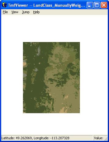
| MajorityMode | Simple Weighted | Simple majority of input samples determines the output value. Input samples are not weighted unless any sample weights are provided manually via SampleWeight parameter. Automatically weight input sample values to preserve the statistical distribution of sample values from the input to the output. Automatic weights are overridden by any weights specified manually via the SampleWeight parameter. | Simple | optional | optional | optional | optional | optional |
| MaxValidValue | number, ? | Maximum value for each channel that will be considered to be valid. Any value greater than this will be considered as missing data. For imagery sources use a comma-separated list: red,green,blue,[,water[,blend]]. For all other sources use a single value. | optional | optional | optional | optional | optional | |
| MinValidValue | number, ? | Minimum value for each channel that will be considered to be valid. Any value less than this will be considered as missing data. For imagery sources use a comma-separated list: red,green,blue,[,water[,blend]]. For all other sources use a single value. | optional | optional | optional | optional | optional | |
| NullValue | number, ? | Sample value for each channel indicating that there is no data in the current pixel. For imagery sources use a comma-separated list: red,green,blue,[,land/water[,blend]]. For all other sources use a single value. Typically NullValue might be set to 255,255,255, as white indicating no data. Also refer to the millenniumimage_water_blend.inf file for an example of using this parameter to reduce the size of BGL files. | optional | optional | optional | optional | optional | |
| SampleWeight.n | value,weight | For majority sampling, apply a manual weight to specific sample values, where n = 1 ? NumberOfWeights | optional | optional | optional | optional | optional | |
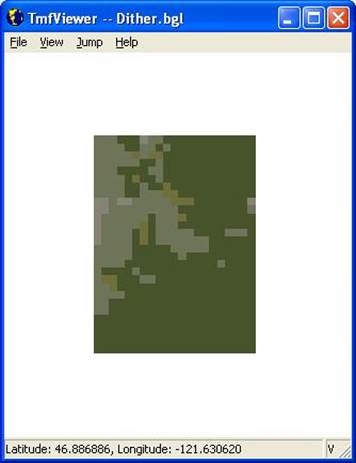
| SamplingMethod | Point Majority Dither Bilinear Gaussian | Simple point sample Majority value within sample window prevails Dither between nearest neighbors when oversampling. Fallback to point sampling when downsampling. Bilinear interpolation Gaussian interpolation | Majority for classification data; Gaussian for continuous data | optional | optional | optional | optional | optional |
| Scale | number, ... | Scale multiplied by each channel before biasing. For imagery sources use a comma-separated list: red,green,blue,[,land/water[,blend]]. For all other sources use a single value. | 1.0 | optional | optional | optional | optional | optional |
| BandGapBytes | integer | Number of bytes between bands (BSQ - Band Sequential layouts only). | 0 | optional | ||||
| BandLayout | BIL BIP BSQ | Band interleaved by line Band interleaved by pixel Band sequential (separate bands) | required | |||||
| BandRowBytes | integer | Number of bytes per band per row | nCols * sizeof( SampleType) | optional | ||||
| ByteOrder | Intel Motorola | Least significant byte first Most significant byte first | required | |||||
| nBands | integer | Number of bands | required | |||||
| SampleType | UINT8 SINT8 UINT16 SINT16 UINT32 SINT32 UINT64 SINT64 FLOAT32 FLOAT64 | 8 bit unsigned integer 8 bit signed integer 16 bit unsigned integer 16 bit signed integer 32 bit unsigned integer 32 bit signed integer 64 bit unsigned integer 64 bit signed integer 32 bit IEEE floating point 64 bit IEEE floating point | required | required | ||||
| SkipBytes | integer | Number of bytes to skip at start of file | 0 | optional | ||||
| TotalRowBytes | integer | Total number of bytes per row | BIL: nBands * BandRowBytes BIP: nCols * nBands * sizeof( SampleType) BSQ: BandRowBytes | optional | ||||
| Month | integer | Month of the year (1-12) associated with Season data sources. | optional | optional | optional | optional | optional | |
| Variation | January February March April May June July August September October November December Day (all months) LightMap or Night All (day and night) | Temporal variation (month or time of day) associated with Imagery data sources. LightMap images are used at night during all months. To associate a single image with more than one temporal variation, use multiple values separated by commas. For example, to use a single image in both January and February, type "Variation = January,February" | optional | optional | optional | optional | optional | |
| VectorAttributeValue.n | whereClause, number whereClause, fieldName | Used by VectorGDB data sources to assign a value to polygons when rasterizing them. The whereClause is a SQL "where clause" that selects the relevant polygon features. To select all features, use an asterisk (*) for the whereClause. The number is the sample value to use when rasterizing the selected polygons. Alternately, a fieldName may be specified that determines the sample value to be assigned to the selected polygons. The first VectorAttributeValue must have a ".1" suffix and additional ones count up from there. For example VectorAttributeValue.1, VectorAttributeValue.2, etc. | required |
Destination Parameters
The destination parameters are all held in a single [Destination] section, and the parameters can be listed in any order.
[Destination] section
| DestFileType | BGL BIP |
Simulator data file Raw BIP file |
BGL | optional |
| DestDir | text | Destination file directory, in quotes. If the directory does not exist, the tool will create it. | required | |
| DestBaseFileName | text | Destination file name without an extension, in quotes. If the file already exists, it will be overwritten. | required | |
| SplitDirLOD | number | Segment the resampled data into multiple destination subdirectories based upon the bounds of cells with the given LOD. | optional | |
| SplitFileLOD | number | Segment the resampled data into multiple destination files based upon the bounds of cells with the given LOD. Must be greater than or equal to DestDirLOD (if used). | optional | |
| GCS (geographic coordinate system, for BIP files only) | WGS84 | World Geodetic System of 1984 | WGS84 | optional |
| QMIDn | Simulator quad mesh identifier (where n is level 0-30). See QMID and LOD Values. | |||
| QMC | Simulator quad mesh coordinate system | |||
| QMIC | Simulator quad mesh integer coordinate system | |||
| NorthLat | number | North limit of sampling region in degrees. | 90 | optional |
| SouthLat | number | South limit of sampling region in degrees. | -90 | optional |
| EastLon | number | East limit of sampling region in degrees. | 180 | optional |
| WestLon | number | West limit of sampling region in degrees. | -180 | optional |
| BoundingCell | level,u,v | QMID of single cell to bound the sampling region, and horizontal and vertical co-ordinates. See QMID and LOD Values. |
optional | |
| MinBoundingCell | level,u,v | QMID of cell forming the northwest bound of the sampling region, and horizontal and vertical co-ordiinates. Must be used with MaxBoundingCell. | optional | |
| MaxBoundingCell | level,u,v | QMID of cell forming the southeast bound of the sampling region, and horizontal and vertical co-ordinates. Must be used with MinBoundingCell. | optional | |
| UseSourceDimensions | 0 or 1 | If set to 1, match the sampling region to the bounds of the data sources. When UseSourceDimensions is enabled with multi-source files, Resample computes the union of the dimensions of all source the files. | 0 | optional |
| CompressionQuality | integer | Quality of compression. A value of 100 indicates lossless compression and best quality. Smaller values indicate higher compression and lower quality. | 100 | optional |
| LOD | [min,]max | Level of detail of each block of samples where LOD + 2 = QMID level. If this parameter is set as LOD=Auto, or LOD=Auto,max or LOD=min,Auto, appropriate levels of detail are chosen to match the resolution of the source data, within the range specified. Using LOD=min,max sets the range definitively. Sometimes it is valuable to create data at a single level of detail (using LOD=N, see Performance Tips for Aerial Imagery). Refer to QMID and LOD Values. |
7 for classification data and imagery. | optional |
| MaxAutoLOD | integer | The maximum allowable LOD that can be selected if LOD=Auto. | optional | |
| FractionBits |
integer |
By default height values are stored as 16 bit signed integers (in meters). If FractionBits is set then the specified number of bits determine the fractional part. For example, if FractionBits is set to 1, then 15 bits hold the interger part and one bit holds the fraction part and an accuracy to 0.5 meters is possible. If it is set to 2 then accuracy to 0.25 meters is possible, and so on. The drawback of setting FractionBits is that it reduces the overall range of possible height values, though only in very mountainous regions, or with a high number of fraction bits set, is this likely to be a factor. For example if FractionBits is set to 3, then height values are stored to 0.125 meter, with a range in height set by the remaining 13 bits of 8192 meters (-4096 to +4096 meters). Height values are always interpreted as signed integers, even if a BaseValue is set. See the examples in the section Using Scaled Elevation Values below. |
0 | optional |
| BaseValue | integer | A value in meters for height, that will be added to all elevation data. This can be used when a very high degree of precision in height is required by setting a substantial number of FractionBits, see Using Scaled Elevation Values. | 0 | optional |
Notes on .inf Files
The Geotiff File Format
Most of the data used by the simulator can be modified using files in the Geotiff file format. In general this is the recommended method for making changes to the default data, because much of the complexity of the parameters for the data is held within the file, which makes resampling using this format quite easy. Another advantage is clearly that the data is viewable with a simple bitmap viewer, such as Microsoft Paint. For full details of this file format, refer to the following document:
Note that the Resample tool interprets all atitudes to be in meters, even if the header of the data file specifies other units. If data is not available in meters, use the Scale parameter to convert to meters (for example: Scale=0.3048 to convert from feet to meters).
Data that can be updated using Geotiff files includes: elevation, land class, water class, and population density. Data that cannot be updated using this format includes region and season data, this information is specific to the simulator, and will need special treatment.
Using Scaled Elevation Values
The simulation supports scaled elevation values. The elevation resampler provides a capability whereby very precise elevation values can be specified at the expense of the range of these values. By default, the resampler expects elevation values to be in increments of one meter. However, with the BaseValue and FractionBits directive, you can specify different scalings for destination data. For example, if you have source data precise to 1/128 meter, then to represent the example data without any loss of accuracy, specify 9 bits for the whole number part and 7 bits for the fraction part, or a 9.7 number. Do this with the following directive:
FractionBits = 7
Since 9 bits are reserved for the whole number part, the range is -512 to 511.984375 meters. This is a fairly narrow range. Unless the area on the earth represented by this data is below 512 meters (and above -512 meters), there would be a problem representing the magnitude of the elevations. An elevation of 1000 meters, for example, cannot be expressed with a "9.7" scaled number. It is outside of the range. To solve this problem, the directive BaseValue can be used to define a "zero point" for the elevation values. For example, if the following is specified:
FractionBits = 7
BaseValue = 1000
A value of zero in the source data indicates a height of 1000 meters. A value of 1 indicates a height of 1000 + 1/128 meter (or 1000.78125), and so on.
Use the FractionBits and BaseValue directives in the [Destination] section, in the [Source] section these parameters have a different, and now deprecated, purpose. The example below shows how to remove a terracing artefact from high resolution data of Mt St Helens using the FractionBits paramater of the [Destination] section.
 |
This image of Mt St Helens is rendered when FractionBits = 0. Note the terracing effect. Mt St Helens is an active volcano in southwest Washington State (height 2550 meters, 8364 feet). Setting the FractionBits parameter to 3 provides a vertical resolution of 0.125m, rather than the default of 1.0m, corrects the terracing artefact. If FractionBits was set to 4, the remaining 12 bits gives a height range of -2048 to +2048 meters, which is not enough to cover the height of Mt St Helens (2550 meters). If this degree of resolution is required, then the BaseValue parameter can be used. Setting BaseValue to 1000 meters in this case would give a range of -1048 to +3048 meters, enough to cover all the elevation data around Mt St Helens. |
QMID and LOD Values
QMID (Quad Mesh Identifier) values are an internal system used to optimize the textures required to represent the Earth, depending on the altitude the aircraft is flying at. Levels 0 and 1 are not used. At level 2 the Earth is divided into six quadrants, three for each hemisphere. Level 3 divides each of the quadrants in the higher level into four, and so on down to level 17 which gives a ratio of one pixel to 1.19 meters. Unfortunately the QMID levels do not match the LOD (Level of detail) levels exactly, there is an offset of 2 between these two indexing systems.
| 2 | 0 | 90 | 0.350194553 | 38913.62 |
| 3 | 1 | 45 | 0.175097276 | 19456.81 |
| 4 | 2 | 22.5 | 0.087548638 | 9728.40 |
| 5 | 3 | 11.25 | 0.043774319 | 4864.20 |
| 6 | 4 | 5.625 | 0.02188716 | 2432.10 |
| 7 | 5 | 2.8125 | 0.01094358 | 1216.05 |
| 8 | 6 | 1.40625 | 0.00547179 | 608.03 |
| 9 | 7 | 0.703125 | 0.002735895 | 304.01 |
| 10 | 8 | 0.3515625 | 0.001367947 | 152.01 |
| 11 | 9 | 0.17578125 | 0.000683974 | 76.00 |
| 12 | 10 | 0.087890625 | 0.000341987 | 38.00 |
| 13 | 11 | 0.043945313 | 0.000170993 | 19.00 |
| 14 | 12 | 0.021972656 | 8.54967E-05 | 9.50 |
| 15 | 13 | 0.010986328 | 4.27484E-05 | 4.75 |
| 16 | 14 | 0.005493164 | 2.13742E-05 | 2.38 |
| 17 | 15 | 0.002746582 | 1.06871E-05 | 1.19 |
| 18 | 16 | 0.001373291 | 5.34354E-06 | 0.59 |
| 19 | 17 | 0.000686646 | 2.67177E-06 | 0.30 |
| 20 | 18 | 0.000343323 | 1.33589E-06 | 0.15 |
| 21 | 19 | 0.000171661 | 6.67943E-07 | 0.07 |
| 22 | 20 | 8.58307E-05 | 3.33972E-07 | 0.04 |
| 23 | 21 | 4.29153E-05 | 1.66986E-07 | 0.02 |
| 24 | 22 | 2.14577E-05 | 8.34929E-08 | 0.01 |
| 25 | 23 | 1.07288E-05 | 4.17464E-08 | 0.00 |
| 26 | 24 | 5.36442E-06 | 2.08732E-08 | 0.00 |
| 27 | 25 | 2.68221E-06 | 1.04366E-08 | 0.00 |
| 28 | 26 | 1.3411E-06 | 5.21831E-09 | 0.00 |
| 29 | 27 | 6.70552E-07 | 2.60915E-09 | 0.00 |
The QMID and LOD grids can be viewed using the TmfViewer tool, for example:
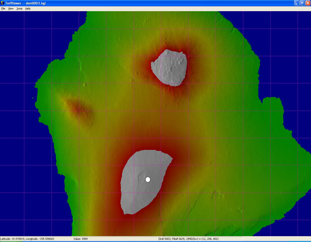
| The following image shows the globe with the QMID level 3 grid. The highlighted area is the base area around Hawaii, which is the dem data that was loaded into the tool. This file is dem0003.bgl in the scenery\0003 folder. |
 |
| The following image shows Hawaii and the QMID level 11 grid. Note the latitude and longitude co-ordinates of the pointer, which is in the grid square marked by the white circle, in the bar bottom right. The QMID level, u and v co-ordinates are in the bar, bottom left: |
 |
| The following image shows Hawaii and the QMID level 12 grid (note the grid squares are one quarter the area of QMID level 11): |
 |
Performance Tips for Aerial Imagery
If aerial photography is being used to replace a large area with detailed imagery, involving the division of the target area into a large number of bgl files, there can be a significant increase in scenery load times. This can be due to an excessive amount of transparency within cells at one or more LOD level. Use the tmfViewer tool to examine the bgl files produced by the Resample tool, and note that transparent areas are shown in medium gray (see the image below).
If there is transparency within a cell at any LOD level, the terrain system has to load in multiple files to piece together the terrain texture for each cell. With a large amount of transparency, and a large number of bgl files containing images, this piecing together can become very time consuming. Minimize transparency within each LOD cell by preparing .inf files that target specific LOD levels. The default Destination parameter LOD=Auto should be changed to provide a minimum and maximum level, or simply one level, that minimizes transparency for the particular LOD settings. This will involve having several .inf files for each section of source data.
The number of bgl files used to hold image data at one level of detail should be reduced by a factor of four for the next level of detail. So, for example, if 16 files are used to hold an area at LOD 14, then four should contain all the imagery at LOD 13, and one at LOD 12. From then on there is no need to have one file for each level of detail, all the lower levels of detail can be placed in one file.
The image shows an an excessive amount of transpareny at one LOD level. If the rest of the cell was also made up of photo-imagery the terrain system would have to piece together the cell from many textures, which would cause a performance issue. 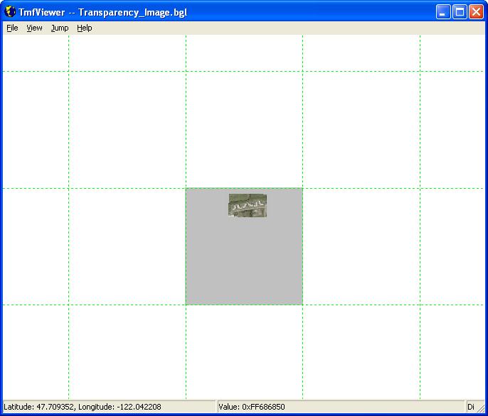
Default land class textures will be used if the terrain system cannot find photo-imagery at LOD13 (5 meters per pixel) or greater detail. This can lead to default textures appearing when photo-imagery is desired. To ensure that the LOD13 requirement is met, consider using LOD=Auto,13 in the [Destination] section of the .inf file. Also be careful with the CompressionQuality setting, change the default of 100 to around 80, and adjust one way or the other to get an acceptable compromise of image quality and size.
Resample Samples
All sample .inf files are in the Terrain SDK/Resample Examples folder. The output from running the samples will be placed in the Terrain SDK/Resample Examples/Output folder. The input is in the Terrain SDK/Resample Examples/SourceData folder, and can be examined just by double-clicking on the files to open them up in an image viewer.
- Sample 1: Replacing Elevation Data
- Sample 2: Creating new Land Classifications
- Sample 3: Creating Custom Terrain Textures
- Sample 4: Custom Terrain Texture with Water and Blend Channels
- Sample 5: Multiple Source and Blend Channels
Sample 1. Replacing Elevation Data
To run this sample, drag the DeathValley_Elevations.inf file onto the Resample tool icon.
Textures for all appropriate levels of detail are created by the Resample tool, and stored in the BGL files. For the Death Valley sample, the tool creates and stores textures only in LODs 2-10. You can confirm this by opening DeathValley_Elevations.bgl in TmfViewer by expanding the "Level of Detail" item on the View menu. When you do this you will notice that only levels 2-10 are enabled in the menu. All the other levels are grayed out because they do not exist in the bgl file. The images below show Death Valley elevation data from QMID level 2 to level 10.
| Death Valley at QMID level 2 |
 |
| Death Valley at QMID level 4 |
 |
| Death Valley at QMID level 6 |
 |
| Death Valley at QMID level 8 |
 |
| Death Valley at QMID level 10 |
 |
Notes on Acquiring Raw Digital Elevation Data
A DEM provides a digital representation of a portion of the earth's elevation points over a two-dimensional surface. A DEM is generated by sampling an array of elevation values derived from topographic maps, aerial photographs, or satellite images.
There are a number of places to get digital elevation data. Most terrain data available for free over the Internet is typically stored in formats such as the USGS DEM (Digital Elevation Model) ASCII, USGS TAR, or USGS Spatial Data Transfer Standard (SDTS) formats. All source data is expected to use WGS84 projection.
For example, this is a link to the USGS 100 meter DEM for the entire United States of America. Just click on the area of DEM you want:
http://edcwww.cr.usgs.gov/glis/hyper/guide/1\_dgr\_demfig/index1m.html
The raw data used when creating terrain must be in a binary file format, with each elevation point (measured in meters above mean sea level) being assigned a 16-bit integer. The resampler supports both LSB (least significant byte first) and MSB (most significant byte first) 16-bit integers.
The USGS DEM and SDTS formats are not compatible with the terrain tools included with this SDK, but there are converters available (free of charge) on websites that convert the data to a compatible binary form. For example, see the read_dem.exe tool that is available for download at http://dbwww.essc.psu.edu/notes/utilities.html. After using this tool, you should be able to run the output DEM data through the Resample tool.
You may find that the source files you acquire come with a header file. This header file provides the information needed for some sections of the .inf file such as the bounding area.
Sample 2: Creating new Land Classifications
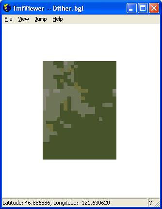
To run these samples, drag theLandClass_AutoWeightedMajority, LandClass_Dither, LandClass_ManualWeightedMajority, LandClass_PointSample and LandClass_SimpleMajority .inf files onto the Resample tool icon. The output can be viewed in TmfViewer, and should look like the images shown below. If an image is not showing in TmfViewer after loading, check the Level of Detail menu, to be sure that one of the appropriate levels of detail has been selected.
| LandClass Auto Weighted Sample | LandClass Dither Sample |
 |
 |
| LandClass Manual Weighted Sample | LandClass Point Sample |
 |
 |
| LandClass Simple Majority Sample | |
 |
Sample 3: Creating Custom Terrain Textures
To run these samples, drag the MillenniumImage and DayNight_Variations .inf files over the Resample tool icon.
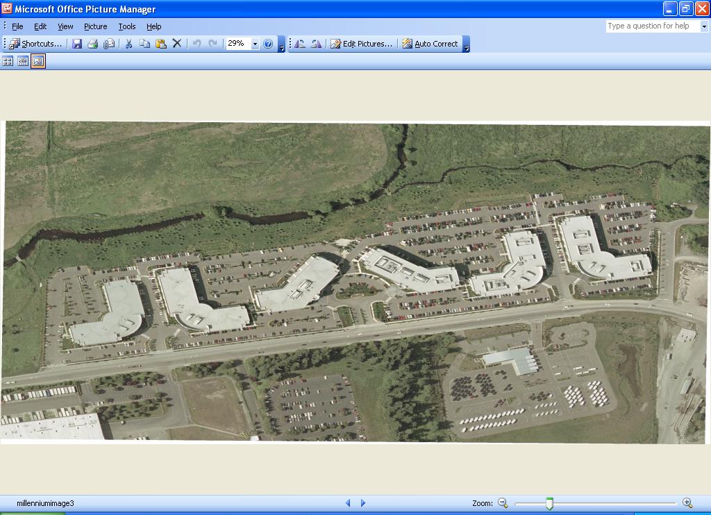
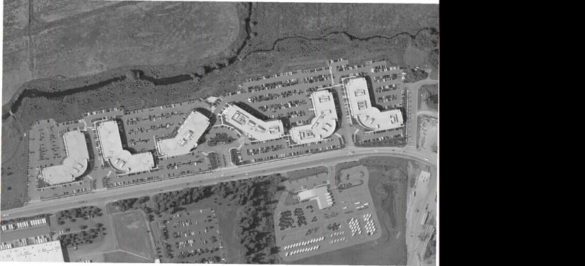
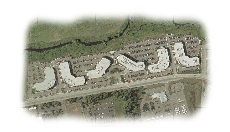
The Millennium sample illustrates a couple of concepts, the use of a GeoTIFF image with Resample, using a source image with transparent "NullValue" pixels, setting the lossy compression quality to 75%, and using an automatic selection for the LOD levels. The Resample tool outputs a range of LODs appropriate for the source image. After the Resample tool finishes, open the resulting .BGL file in TmfViewer to view the imagery. You can also drop the .BGL file in Microsoft ESP/1.0/Addon Scenery/scenery to view it in the simulation. The imagery will appear near N47.68, W122.1.
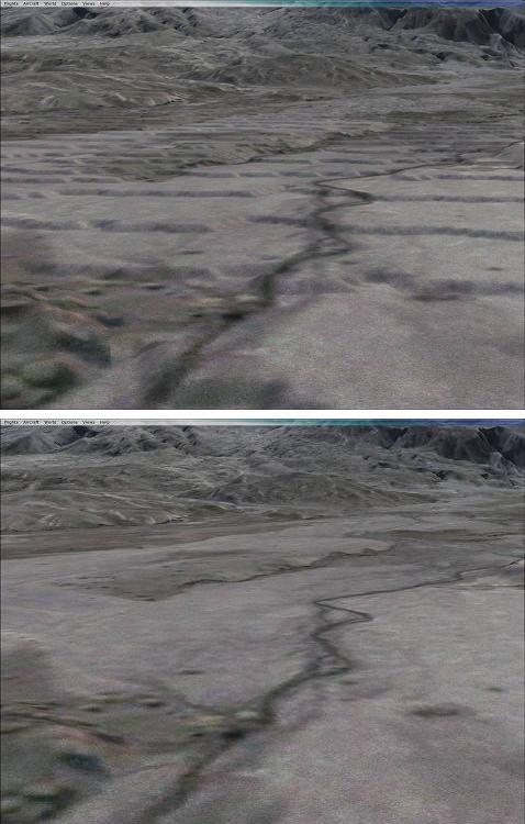
The DayNight_Variations sample shows how two different textures apply during different hours of the day. It also shows the use of multiple source files, and the providing of co-ordinates within the .inf file, rather than the raw data. The resulting textures can be viewed in TmfViewer, or in the simulation if the bgl file is moved to Addon Scenery/scenery. In TmfViewer chose different Levels of Detail to view the image, and check on Night in the Seasons/Variations submenu to see the nighttime image. To view the imagery in the simulation, use the Map feature and enter the location: N0 W122.308. You will be flying around the open Pacific and the images will be rendered onto the sea (see the screen shots below).
These samples show how to add custom satellite or aerial imagery to the terrain in ESP. These are simply the textures used to render onto the terrain, to add buildings and trees to custom textures, follow the directions in the Autogen annotation document. Areas like New York City, Chicago, and Las Vegas were created using the methods discussed here, and in the Autogen document.
| Millennium Buildings: note the white space around the edges is removed by setting the NullValue parameter to 255,255,255. |
 |
| Day |
 |
| Night |
 |
| Dawn |
 |
| Dusk: note the merging of both the Day and Night variations |
 |
Notes on Acquiring Raw Terrain Imagery
More than likely, the image you want to use will be an aerial or satellite photo. The raw image must be either a 24-bit per pixel Windows .bmp file or a 32-bit per pixel Targa .tga file. For some file formats, you can use Imagetool to convert the image into the desired format. It is assumed that the image has been projected to the WGS84 Latitude/Longitude datum. The latitude and longitude of the northwest corner of the image must be known as well as the spacing (in decimal degrees) between the image pixels.
To add reflective water effects to an image, you must use the 32-bit per pixel Targa .tga format. The resampler tool uses the 8-bit alpha channel of the image to determine the location of water and land in the image. The alpha value of water and land pixels must be 0 and 255 respectively.
The north/south extent of each terrain texture pixel is about 1.19 meters in ESP. The resampling process will filter the raw image to the right size.
• If the raw image is more than 1.19 meters per pixel (low resolution), the final result may appear blurry.
• If the raw image is less than 1.19 meters per pixel (high resolution), some fine details might be lost.
Sample 4: Custom Terrain Texture with Water and Blend Channels
To run this sample drag the MilleniumImage_water_blend.inffile over the Resample tool icon.
The sample shows the use of the water and blend channels, and can be compared with the Millennium Buildings in Sample 3.
| The following image shows the source: Millennium_water_blend.tif |
 |
| The following image shows the Millennium_water_blend.bgl file, loaded into TMFViewer, with the Level of Detail set to 17. |
 |
| The following image shows the Millennium_water_blend.bgl file, loaded into TMFViewer, with the missing data and water mask menu items selected. |
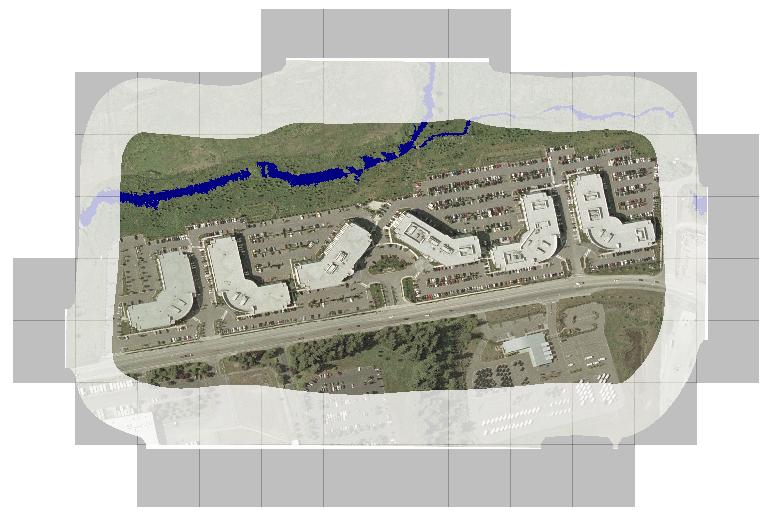 |
Sample 5: Multiple Source and Blend Channels
This sample shows how to read the land/water mask and/or blend mask from separate files from the main color channels. The land/water mask only controls the location of water effects (such as reflections, specular highlights and animated swells) and has no effect on the base color of the texture. This enables the color of the source image to be preserved while still applying the water effects to it.
To run this sample drag the Multichannel_Multisource.inf file over the Resample tool icon. The location of the sample terrain is at Latitude 0.0, Longitude -122.308, which can be viewed after placing the bgl output file into the simulation. Examine the Blend Mask and LandWater Mask files and the following screen shot taken from within ESP. Also note that a good example of this technique is used for the island of St. Maarten (go to the airport TNCM and view the coastline).
.jpg)
.jpg)
 |
Place the new Files in ESP
The easiest way to add a new .bgl file to ESP is to copy it into the Addon Scenery\Scenery directory. Files in this directory are treated as higher priority than those in other directories, so new terrain data here will be rendered in preference to lower priority data elsewhere. However, for complex new additional scenery, it is probably more useful to create a folder for the custom scenery area. This will enable a user to select and deselect the scenery using the Scenery Library dialog.
To create the appropriate directories:
- Create a new scenery area folder, with an appropriate name. Within each scenery area, create two subdirectories: Scenery and Texture.
- Place any .bgl files into the Scenery directory.
- Place any necessary .bmp files into the Texture directory.
- Run ESP and choose Scenery Library under the Settings tab.
- Click the Add Area button and fill in the blanks. The new scenery area will not be visible in ESP until you restart the program.
The final step is to view the new data within ESP, and go back and repeat the resampling steps if it is not quite right (possibly resampling to a higher or lower resolution).
Appendix I: The World Coordinate System
One of the most powerful features of BGL is that everything is based on a world coordinate system that is spherical and very much like latitude/longitude.
In ESP, the earth is defined as an “oblate spheroid,” an ellipse rotated about its minor axis. In terms of shape, it's much like a sphere that is a little bit fat around the equator. In ESP, the earth has the following dimensions:
• Equatorial diameter=12756.27 km
• Equatorial circumference=40075.0 km
• Polar diameter=12734.62 km
• Polar circumference=40007.0 km
Unlike other 3-D graphics systems (rectilinear systems that overlay a square grid over a map that is really a portion of a sphere), the position of scenery in BGL is specified in world coordinates. The following table includes the elements of the world coordinate system used by BGL and ESP to specify position in the world.
| Longitude | 0 at 0° longitude. East is positive; west is negative with overflow wrap at 180°. |
| Altitude | 0 at sea level. Positive is up; negative is down. |
| Latitude | 0 at equator. Positive is north; negative is south. |
Although the position of objects on the earth is specified in the world coordinate system, actual design work is done in smaller rectilinear coordinate systems placed with their centers at a given world coordinate.
The Object Coordinate System
The object coordinate system is used to design scenery. The object coordinate system is based on the X, Y, Z concept of design space. The rectilinear, 3-D X, Y, Z coordinate system is set up with its center, X=Y=Z=0, at the specified latitude, longitude, and altitude. The Z-axis aligns with true north (parallel to lines of longitude), the X-axis aligns with east (parallel to lines of latitude), and the Y-axis aligns with altitude. You can define points, lines, and polygons within the X, Y, Z design space.
The X, Y, and Z-axes each have a range of +/-32767 (16-bit linear design space). The size that each unit along the axes represents depends on the scale factor. The scale factor can range from less than 1 millimeter per unit to 32768 meters per unit.
The object design system creates some interesting design problems not unlike those in the real world. For example, a 1 mile square section of land in the northern hemisphere encompasses more longitude at its northern edge because this edge is further north on the sphere. Conversely, a "square" piece of land that has its east and west borders precisely aligned with lines of longitude and its north and south borders aligned with lines of latitude is not really square because its north edge is shorter than its south edge. When aligning many square pieces on the surface of the earth, the result is either some pieces that are not square or small gaps between some pieces.
The Coordinate System, Basic Principles
The coordinate systems used in ESP are left-hand, 3-D, and rectilinear. Objects are located in X,Y,Z 3-D space and are moved in the X,Y, and Z directions using translation. The following table describes how this directional translation of an object occurs in the world as well as on the screen.
| +X | West to east | Left to right |
| +Y | Increasing altitude | Bottom to top |
| +Z | South to north | Into the screen |
ESP directional conventions include the following:
• The surface of the earth is laid out on the X-Z plane.
• Northerly movement is in the positive Z direction.
• Easterly movement is in the positive X direction.
• Increasing altitude movement is in the positive Y direction.
• World directional movement corresponds to display screen directional movement when the viewer is facing north. For example, an easterly moving object moves to the right across the screen when the viewer is facing north.
ESP uses Euler angles for rotations; first heading is applied, then pitch, and finally bank. The following table describes the rotational conventions.
| +Heading, rotate about the Y-axis | Rotate to the right; 0° is north | Object moves left as heading increases. |
| +Pitch, rotate about the heading-rotated X-axis | Nose down | Object moves upward (+Y) as pitch increases. |
| +Bank, rotate about the heading-rotated and pitched Z-axis | Rotate counter-clockwise | The object rotates clockwise as bank increases. |
Directional translation and rotation are applied to objects before they are projected. The order in which directional translation and rotation are applied makes a difference because the rotations have the effect of "rotating" the coordinate system. Translation and rotation are performed in the following order:
1. Translate X.
2. Translate Y.
3. Translate Z.
4. Rotate heading (about the Y-axis).
5. Rotate pitch (about the heading-rotated X-axis).
6. Rotate bank (about the heading-rotated and pitched Z-axis).
Appendix II: The Naming Convention for Terrain Textures
This section describes the naming convention used by ESP for terrain (land based) textures. The textures are found in the Microsoft ESP/1.0/scenery/World/texture folder. The naming convention follows the format:
000X2SU1
| 000 | The texture number (000, 001, and so on). |
| X | Region (A through X), see Regions. |
| 2 | Reserved, must always be 2. |
| SU | Season, one of: spring (SP), summer (SU), fall (FA), winter (WI), hard winter (HW), night texture (LM), or Autogen annotation (AN). See Seasons. |
| 1 | Variation (1, 2, 3, and so on). |
 |