Types of parallelism
A second consideration in developing distributed programs involves specifying the type of parallelism, data or graph parallelism. The data parallelism design emphasizes the distributed nature of data and spreads it across multiple machines. Computation, meanwhile, can remain the same among all nodes and be applied on different data. Alternately, tasks on different machines can perform different computational tasks. When the tasks are identical, we classify the distributed program as single program, multiple data (SPMD); otherwise, we categorize it as multiple program, multiple data (MPMD).
The basic idea of data parallelism is simple: by distributing a large file across multiple machines, it becomes possible to access and process different parts of the file in parallel. As discussed in an earlier module, one popular technique for distributing data is file striping, in which a single file is partitioned and distributed across multiple servers. Another form of data parallelism is to distribute whole files (without partitioning) across machines, especially if files are small and their contained data exhibits very irregular structures. We note that data can be distributed among distributed tasks either explicitly, by using message passing, or implicitly, by using shared memory, assuming that the underlying distributed system supports shared memory.
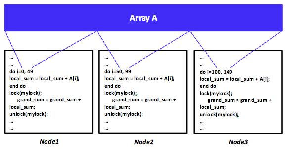
Figure 9: An SPMD distributed program using the shared-memory programming model
Data parallelism is achieved when each node runs one or many tasks on different pieces of distributed data. As a specific example, assume array A is shared among three machines in a distributed shared-memory system. Consider also a distributed program that simply adds all elements of array A. It is possible to command machines 1, 2, and 3 to run the addition task, each on one-third of array A, or 50 elements, as shown in Figure 9. The data can be allocated across tasks using the shared-memory programming model, which requires a synchronization mechanism. Clearly, such a program is SPMD. In contrast, array A can also be distributed evenly (using message passing) by a (master) task among three machines, including the master's machine, as shown in Figure 10. Each machine will run the addition task independently; nonetheless, summation results will have to be eventually aggregated at the master task in order to generate a grand total. In such a scenario, every task is similar in a sense that it is performing the same addition operation, yet on a different part of array A. The master task, however, is also distributing data to all tasks and aggregating summation results, thus making it slightly different from the other two tasks. Clearly, this makes the program MPMD. As will be discussed in a later unit about MapReduce, MapReduce uses data parallelism with MPMD programs.
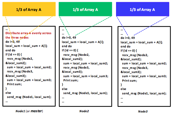
Figure 10: An MPMD distributed program using the message-passing programming model
Graph parallelism, on the other hand, focuses on distributing computation as opposed to data. Most distributed programs actually fall somewhere on a continuum between the two forms. Graph parallelism is widely used in many domains such as machine learning, data mining, physics, and electronic circuit design. Many problems in these domains can be modeled as graphs in which vertices represent computations and edges encode data dependencies or communications. Recall that a graph $G$ is a pair, $(V, E)$, where $V$ is a finite set of vertices and $E$ is a finite set of pairwise relationships, $E \subset (V \times V)$, called edges. Weights can be associated with vertices and edges to indicate the amount of work at each vertex and the communication data on each edge.
Consider a classical problem from circuit design: the common goal of keeping certain pins of several components electrically equal by wiring them together. If we assume $n$ pins, then an arrangement of $(n - 1)$ wires, each connecting two pins, can be employed. Of all such arrangements, the one requiring the minimum number of wires is normally the most desirable. Obviously, this wiring problem can be modeled as a graph problem. In particular, each pin can be represented as a vertex, and each interconnection between a pair of pins, $(u, v)$, can be represented as an edge. A weight, $w(u, v)$, can be set between $u$ and $v$ to encode the cost (the amount of wires needed) to connect $u$ and $v$. The problem becomes how to find an acyclic subset, $S$, of edges, $E$, that connects all the vertices, $V$, and whose total weight,
$$ w(S) = \Sigma_{(u, v)\in S} w(u, v) $$
is the minimum.
As $S$ is acyclic and fully connected, it must result in a tree known as the minimum spanning tree. Consequently, solving the wiring problem morphs into solving the minimum spanning tree problem, a classical problem that is solvable with algorithms like Kruskal's and Prim's.
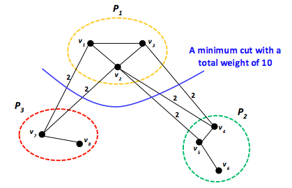
Figure 11: A graph partitioned using the edge-cut metric
Once modeled as a graph, a program can be distributed over machines in a distributed system using a graph-partitioning technique, which involves dividing the work (vertices) over distributed nodes for efficient distributed computation. As with data parallelism, the basic idea is simple: by distributing a large graph across multiple machines, it becomes possible to process different parts of the graph in parallel, resulting in a graph-parallel design. The standard objective of graph partitioning is to distribute work uniformly over p processors by partitioning the vertices into p equally weighted partitions while minimizing internode communication reflected by edges. Such an objective is typically referred to as the standard edge-cut metric. While the graph partitioning problem is NP-hard, heuristics can achieve near optimal solutions. As a specific example, Figure 11 demonstrates three partitions, $P_{1}$, $P_{2}$, and $P_{3}$, at which vertices $ \lbrace v_{1}, \cdots, v_{8} \rbrace $ are divided using the edge-cut metric. Each edge has a weight of two, corresponding to one unit of data communicated in each direction. Consequently, the total weight of the shown edge cut is 10. Other cuts will result in more communication traffic. Clearly, for communication-intensive applications, graph partitioning is critical and can play a dramatic role in dictating the overall application performance. Both Pregel and GraphLab employ graph partitioning, and we further discuss each in later units.
References
- T. H. Cormen, C. E. Leiserson, R. L. Rivest, and C. Stein (July 31, 2009). Introduction to Algorithms MIT Press, Third Edition
- B. Hendrickson and T. G. Kolda (2000). Graph Partitioning Models for Parallel Computing Parallel Computing
- M. R. Garey, D. S. Johnson, and L. Stockmeyer (1976). Some Simplified NP-Complete Graph Problems Theoretical Computer Science
- B. Hendrickson and R. Leland (1995). The Chaco User's Guide Version 2.0 Technical Report SAND95-2344, Sandia National Laboratories
- G. Karypis and V. Kumar (1998). A Fast and High Quality Multilevel Scheme for Partitioning Irregular Graphs SIAM Journal on Scientific Computing