Exercise - Distribute multitenant tables - Training

15 minutes

With the tables in the Tailspin Toys database now prepared for distribution, you're ready to scale the database horizontally and distribute the tables. In this exercise, you scale your single-node database to a multi-node cluster, and then distribute the table data across the nodes by using a combination of distribution methods to minimize the impact of the database changes on the Tailspin Toys multitenant SaaS application. You also execute several popular queries from the multitenant SaaS application throughout the process to measure the impact of your changes on query execution time at various stages.

Scale the database

Scaling an Azure Cosmos DB for PostgreSQL database can be done quickly via the Azure portal. Typically, a database can be scaled without downtime. However, going from a single-node database to a multi-node cluster might require minimal downtime if the coordinator node's compute core and storage sizes change. When you are on a multi-node cluster, you can scale without downtime. It's also important to note that after you go from single-node to multi-node, you can't go back to single-node.

In the Azure portal, go to your Azure Cosmos DB for PostgreSQL Cluster resource.
On the left menu under Settings, select Scale. On the Scale pane, expand the Node count dropdown, and then select 2 nodes from the list.

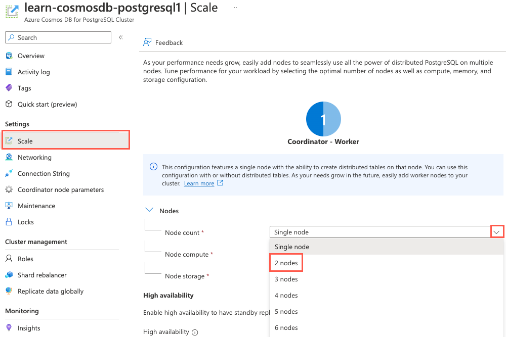
Migrating to a multi-node cluster splits the coordinator and workers onto separate nodes. The node count dropdown indicates the number of worker nodes, so selecting 2 nodes create two worker nodes in addition to the coordinator node.
Select Save to transition the database from a single-node cluster to a multi-node cluster.

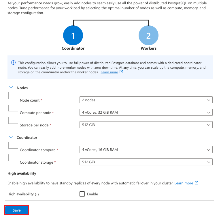
The compute and storage sizes that you selected when you set up the development database for Tailspin Toys are compatible with a multi-node cluster, so scaling the database doesn't cause any database downtime. The scaling process takes several minutes to complete, so you can move on to the next task while it is in progress.

Enable citus_stat_statements monitoring

Queries statistics against PostgreSQL databases are maintained in the pg_stat_statements view. When you transition to a multi-node distributed database, the Citus extension provides another view named citus_stat_statements, which includes the partition key, making it much more helpful in multitenant databases. The citus_stat_statements view should be enabled by default in your database, but it's a good idea to verify it's turned on, and if not, enable it.

To check whether monitoring is turned on, you must select the citus.stat_statements_track setting on your coordinator node. Run the following query to check whether Citus statistics tracking is enabled:
```
show citus.stat_statements_track;
```
If the citus.stat_statements_track setting is all, you can skip to the next section and connect to your database. Otherwise, proceed to the next step to enable tracking.
On your Azure Cosmos DB for PostgreSQL Cluster resource, on the left menu under Settings, select Coordinator node parameters. On the Coordinator node parameters pane, enter citus.stat in the filter box and change the value of citus.stat_statements_track to ALL. If the value is already ALL, select None, and then choose ALL again to enable the Save button.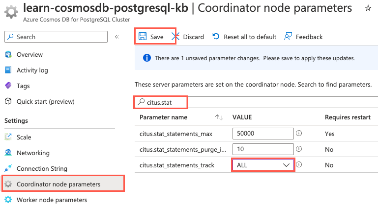
Select Save.
After the updated setting is saved, rerun the verification query:
```
show citus.stat_statements_track;
```

Ensure that the output now displays all:

 citus.stat_statements_track 
-----------------------------
 all

Connect to the database by using psql in Azure Cloud Shell

You use psql at the command prompt to distribute the tables in your database. psql is a command-line tool that allows you to interactively issue queries to a PostgreSQL database and view the query results.

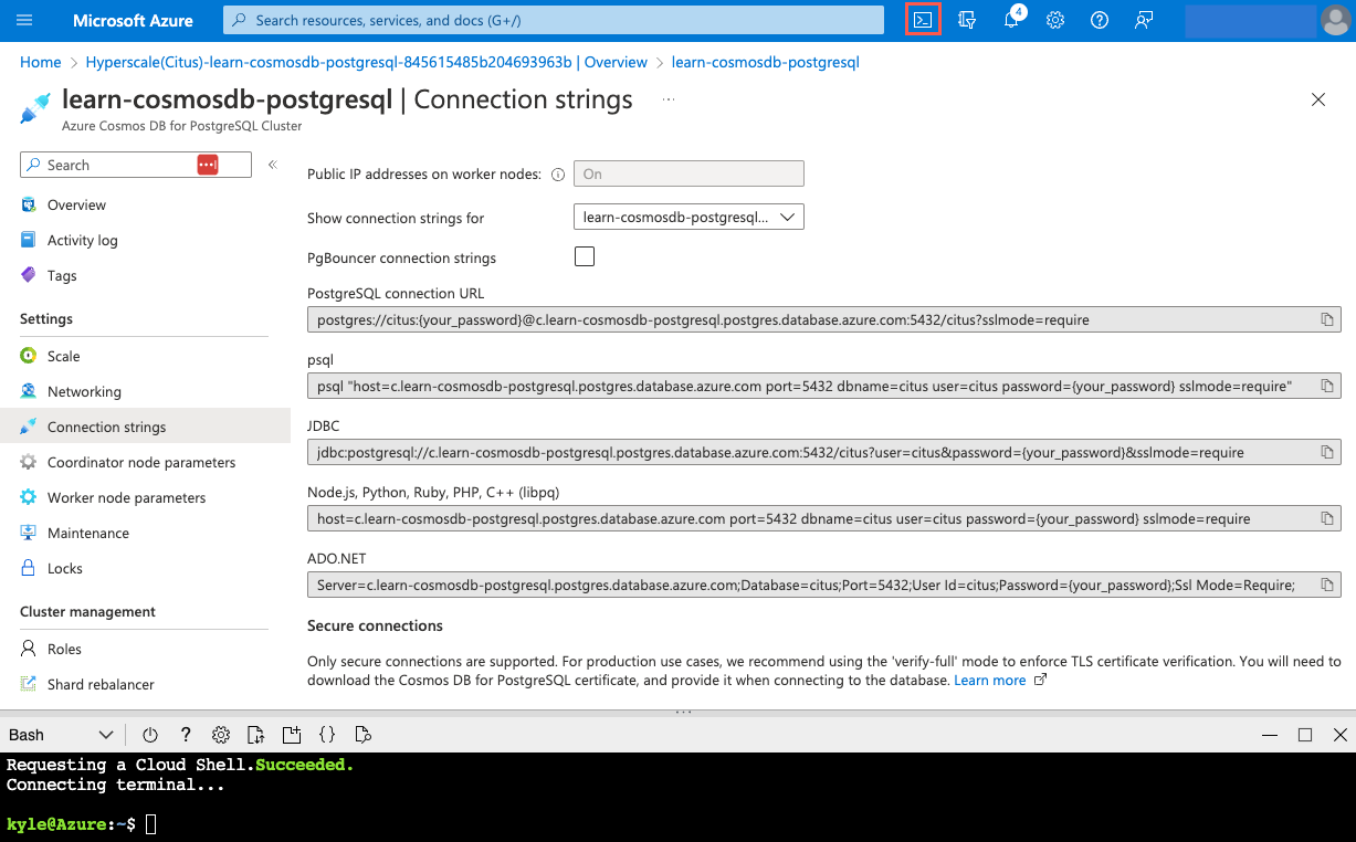
On your Azure Cosmos DB for PostgreSQL resource in the Azure portal, on the left menu under Settings, select Connection strings. Then copy the connection string that's labeled psql.
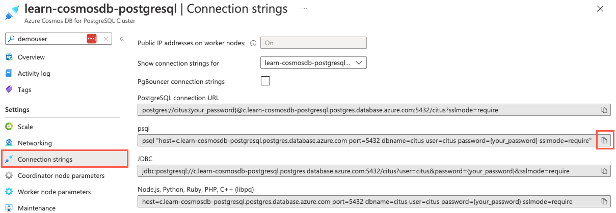
Paste the connection string into a text editor like Notepad. Replace the {your_password} token with the password that you created for the citus user when you created your cluster. Copy the updated connection string to use later.
On the Connection strings pane in the Azure portal, open an Azure Cloud Shell dialog by selecting the Cloud Shell icon in the global controls in the Azure portal.

Cloud Shell opens as an embedded panel at the bottom of your browser window. Alternatively, you can open Azure Cloud Shell in a new browser tab.
In the Cloud Shell pane, ensure that Bash is selected for the environment, and then use the psql command-line utility to connect to your database. Paste your updated connection string (the one that contains your correct password) at the command prompt in Cloud Shell, and then run the command. The command looks similar to the following example:
```
psql "host=c.learn-cosmosdb-postgresql.postgres.database.azure.com port=5432 dbname=citus user=citus password={your_password} sslmode=require"
```

Benchmark query execution times before table distribution

Before you distribute any tables in the database, you want to take baseline measurements on execution times for a few popular queries from the Tailspin Toys multitenant SaaS application. These measurements help you understand the impact of table distribution on query performance.

In the Cloud Shell pane, enable the display of query execution times by running the following from the Citus prompt:
```
\timing
```
As you execute each of the following queries, record its execution time for comparison throughout the table distribution process.
The first query you want to examine retrieves the list of available products for an individual store. This query involves only the products table, and it filters on store_id. Execute the following and record the execution time:
```
-- List products by store
SELECT p.product_id, p.name FROM stores AS s
INNER JOIN products AS p ON s.store_id = p.store_id
WHERE s.store_id = 336;
```

The second query you want to measure is slightly more complex, querying for the top five products sold by a store. It includes aggregations that sum up the total quantity of each item sold and count the number of orders that contain the product. Run the query and record the execution time:

-- 5 most ordered products by store
SELECT p.product_id,
    p.name,
    SUM(l.quantity) AS total_ordered,
    COUNT(p.product_id) AS count_of_orders_containing_product
FROM products AS p
INNER JOIN line_items AS l ON p.store_id = l.store_id AND p.product_id = l.product_id
WHERE p.store_id = 5
GROUP BY p.store_id, p.product_id
ORDER BY total_ordered DESC
LIMIT 5;

The last application query you want to evaluate retrieves averages for the number of items purchased, number of line items, and order total for a store. Execute the query and record its execution time:

-- Average order amounts by store
WITH order_amounts AS (
    SELECT store_id, order_id, SUM(quantity) AS total_quantity, COUNT(*) AS order_lines, SUM(line_amount) AS order_amount
    FROM line_items
    WHERE store_id = 5
    GROUP BY store_id, order_id
)
SELECT s.name,
    AVG(o.total_quantity) AS avg_quantity,
    AVG(o.order_lines) AS avg_order_lines,
    AVG(o.order_amount) AS avg_order_amount
FROM stores AS s
INNER JOIN order_amounts AS o ON s.store_id = o.store_id
WHERE s.store_id = 5
GROUP BY s.store_id;

Tailspin Toys uses this final query for internal analytics. The query aggregates data across all stores and calculates each store's total number of orders, the average dollar amount of each order, and their total sales. Execute the cross-tenant query and record the execution time:
```
-- Internal cross-tenant aggregation
SELECT s.store_id,
    s.name,
    COUNT(l.order_id) AS order_count,
    AVG(line_amount) AS avg_order_amount,
    SUM(l.line_amount) AS total_sales
FROM line_items AS l
INNER JOIN stores AS s ON l.store_id = s.store_id
GROUP BY s.store_id
ORDER BY total_sales DESC
LIMIT 25;
```
Most queries in multitenant SaaS applications are for a single tenant. Still, SaaS providers might run cross-tenant queries to understand how the application is used across tenants or for other purposes, such as to generate data for internal analytics. Understanding the impact of distributing table data across nodes on cross-tenant queries is also an essential metric to capture.

Distribute the stores and products tables

In a single-node nondistributed database, all tables are located on the coordinator node. Horizontally scaling the database to a multi-node cluster doesn't automatically partition data across the new worker nodes. Next, you need to distribute the tables. Start with the stores and products tables.

When the database scaling operation finishes, you want to distribute the stores table first. This table is small and doesn't receive many updates, so you can use create_distributed_table() to handle distribution. At the Citus command prompt in your open Cloud Shell pane, run the following code:
```
SELECT create_distributed_table('stores', 'store_id');
```
You can use the same method to distribute the products table that you used for stores. Similarly, this table is updated less frequently, so the risk of affecting users in the SaaS application is low. This time, the colocate_with option is specified to inform the create_distributed_table() function to explicitly place data with the same distribution key from both tables onto the same node in the cluster:
```
SELECT create_distributed_table('products', 'store_id', colocate_with => 'stores');
```

Reevaluate query execution times

Neither of the distribution functions that are available in Azure Cosmos DB for PostgreSQL works within transactions, so some time elapses between when the first tables and the last tables are distributed. To understand the potential impact of having a mix of local and distributed tables, you want to rerun the application queries that you used in the preceding sections to see if query times are affected by being in this state.

Execute the query to retrieve the products list for a store again, and record the execution time:

-- List products by store
SELECT p.product_id, p.name FROM stores AS s
INNER JOIN products AS p ON s.store_id = p.store_id
WHERE s.store_id = 336;

Rerun the query that retrieves the top five products sold by a store, and document the query's execution time:

-- 5 most ordered products by store
SELECT p.product_id,
    p.name,
    SUM(l.quantity) AS total_ordered,
    COUNT(p.product_id) AS count_of_orders_containing_product
FROM products AS p
INNER JOIN line_items AS l ON p.store_id = l.store_id AND p.product_id = l.product_id
WHERE p.store_id = 5
GROUP BY p.store_id, p.product_id
ORDER BY total_ordered DESC
LIMIT 5;

Execute the average order amount query again, and record the execution time:

-- Average order amounts by store
WITH order_amounts AS (
    SELECT store_id, order_id, SUM(quantity) AS total_quantity, COUNT(*) AS order_lines, SUM(line_amount) AS order_amount
    FROM line_items
    WHERE store_id = 5
    GROUP BY store_id, order_id
)
SELECT s.name,
    AVG(o.total_quantity) AS avg_quantity,
    AVG(o.order_lines) AS avg_order_lines,
    AVG(o.order_amount) AS avg_order_amount
FROM stores AS s
INNER JOIN order_amounts AS o ON s.store_id = o.store_id
WHERE s.store_id = 5
GROUP BY s.store_id;

Run the Tailspin Toys internal cross-tenant aggregation query again, and record the execution time:

-- Internal cross-tenant aggregation
SELECT s.store_id,
    s.name,
    COUNT(l.order_id) AS order_count,
    AVG(line_amount) AS avg_order_amount,
    SUM(l.line_amount) AS total_sales
FROM line_items AS l
INNER JOIN stores AS s ON l.store_id = s.store_id
GROUP BY s.store_id
ORDER BY total_sales DESC
LIMIT 25;

You'll notice a significant increase in the execution time of this query.

Distribute the remaining tables

You've seen that having some of your tables distributed while other tables aren't distributed can affect the performance of queries that join data between tables in different distribution states or read data across tenants. However, you still need to inspect how those queries perform after all tables have been distributed.

Using create_distributed_table() blocks write transactions while table data is being distributed, which might negatively affect perceived application performance. When distributing write-heavy tables in a production environment, it's safer to use created_distributed_table_concurrently() and allow table writes to continue.

To distribute the orders and line_items tables, use the create_distributed_table_concurrently() function to prevent blocking incoming table writes and to minimize application disruption. That function, however, doesn't allow foreign key constraints to exist while distributing the table, so first, you must drop any foreign key constraints on each table to be distributed.

To distribute the orders table, first drop all foreign key constraints that are associated with the table:

BEGIN;

-- Drop the foreign key to the stores table
ALTER TABLE orders
    DROP CONSTRAINT orders_store_id_fkey;

-- Drop the foreign key reference in the line_items table
ALTER TABLE line_items
    DROP CONSTRAINT line_items_orders_fkey;

COMMIT;

When the foreign key references have been removed, you can use create_distributed_table_concurrently() to distribute the orders table:
```
SELECT create_distributed_table_concurrently('orders', 'store_id');
```
Using the create_distributed_table_concurrently() function takes longer than distributing by using create_distributed_table(). This increase in time to execute is primarily because concurrently distributing a table allows table write operations to continue. Distribution is interrupted by any incoming table inserts and updates.

If you receive an error when you run this step, rerun the query to try again.
The last step for the orders table is to re-create the foreign key constraints to tables that have already been distributed, which is only the stores table in this case.
```
ALTER TABLE orders
    ADD CONSTRAINT orders_store_id_fkey FOREIGN KEY (store_id) REFERENCES stores (store_id);
```
You might notice that this command didn't re-create the foreign key constraint between line_items and orders that you dropped in step 1. To avoid errors, you'll re-create that relationship after you distribute line_items.
Before you distribute the line_items table, open the Azure Cloud Shell in a second web browser or tab. You use this second Cloud Shell window to examine how table writes are handled when you use create_distributed_table_concurrently().
In the new Cloud Shell window, ensure that Bash is selected for the environment, then use the psql command-line utility to connect to your database, as you've done previously. Paste your updated connection string (the one that contains your correct password) at the command prompt in Cloud Shell. Run the command, which should look similar to the following example:
```
psql "host=c.learn-cosmosdb-postgresql.postgres.database.azure.com port=5432 dbname=citus user=citus password={your_password} sslmode=require"
```

You can now distribute the line_items table in the same fashion as the orders table. Return to the Cloud Shell pane at the bottom of the Azure portal window. Copy and paste the following code to drop any foreign key references, distribute the table, and then re-create the table relationships:

ALTER TABLE line_items
    DROP CONSTRAINT line_items_products_fkey,
    DROP CONSTRAINT line_items_store_id_fkey;

SELECT create_distributed_table_concurrently('line_items', 'store_id');

-- Re-create a foreign key to the stores table
ALTER TABLE line_items
    ADD CONSTRAINT line_items_store_id_fkey FOREIGN KEY (store_id) REFERENCES stores (store_id);

-- Re-create the foreign key to the orders table
ALTER TABLE line_items
    ADD CONSTRAINT line_items_orders_fkey FOREIGN KEY (store_id, order_id) REFERENCES orders (store_id, order_id);

-- Re-create the foreign key to the products table
ALTER TABLE line_items
    ADD CONSTRAINT line_items_products_fkey FOREIGN KEY (store_id, product_id) REFERENCES products (store_id, product_id);

After you start the commands, return to your second open Cloud Shell window and run the following command to look for any table locks:
```
SELECT wait_event_type, count(*)
    FROM pg_stat_activity
WHERE state != 'idle'
GROUP BY 1
ORDER BY 2 DESC;
```
You'll likely need to rerun this query multiple times until a lock appears in the output. It looks similar to the following example:
```
 wait_event_type | count 
-----------------+-------
 Client          |     5
                 |     1
 Lock            |     1
```
When you see a Lock line, run \x at the command prompt to switch to the extended view so that the query output is easier to read.
After you enable the extended view, execute the following query to examine the lock details:
```
SELECT * FROM citus_lock_waits;
```

Examine the output of the query, which should look similar to the following example:

-[ RECORD 1 ]-------------------------+---------------------------------------------------------------------------------------------------
waiting_gpid                          | 10000001997
blocking_gpid                         | 10000019151
blocked_statement                     | SELECT create_distributed_table_concurrently('line_items', 'store_id', colocate_with => 'stores');
current_statement_in_blocking_process | SELECT create_orders(20000);
waiting_nodeid                        | 1
blocking_nodeid                       | 1

The citus_lock_waits output reveals that the create_distribute_table_concurrently process is blocked by the write operations in create_orders. This information confirms that running the distribution process concurrently allows write operations to continue and indicates why the distribution process takes longer to complete.

You can now close the new Cloud Shell window, because you no longer need it. Return to the original Cloud Shell pane at the bottom of the Azure portal window.
To view details about your distributed tables, you can query the citus_tables metadata table:
```
SELECT * FROM citus_tables;
```

Inspect the output from the query, noting the colocation_id and shard_count for each table:

 table_name | citus_table_type | distribution_column | colocation_id | table_size | shard_count
------------+------------------+---------------------+---------------+------------+-------------
 line_items | distributed      | store_id            |             2 | 465 MB     |          32
 orders     | distributed      | store_id            |             2 | 228 MB     |          32
 products   | distributed      | store_id            |             2 | 6616 kB    |          32
 stores     | distributed      | store_id            |             2 | 1024 kB    |          32

Related data from each table has been colocated, and each table is now distributed across 32 shards.

If you want to view how the shards are distributed across the nodes in your cluster, you can run the following query against the citus_shards view:

SELECT table_name, nodename, COUNT(shardid) AS shard_count, SUM(shard_size) AS size
FROM citus_shards
GROUP BY table_name, nodename 
ORDER BY table_name;

Measure post-distribution query execution times

After you distribute all of your database tables, you want to take final execution time measurements to understand the impact of table distribution on query performance.

Ensure that the display of query execution times is displayed in the Cloud Shell window. Run \timing at the Citus prompt if it isn't.

Execute the query to retrieve the products list for a store again, and note the execution time:

-- List products by store
SELECT p.product_id, p.name FROM stores AS s
INNER JOIN products AS p ON s.store_id = p.store_id
WHERE s.store_id = 336;

Rerun the query that retrieves the top five products sold by a store, and record the execution time:

-- 5 most ordered products by store
SELECT p.product_id,
    p.name,
    SUM(l.quantity) AS total_ordered,
    COUNT(p.product_id) AS count_of_orders_containing_product
FROM products AS p
INNER JOIN line_items AS l ON p.store_id = l.store_id AND p.product_id = l.product_id
WHERE p.store_id = 5
GROUP BY p.store_id, p.product_id
ORDER BY total_ordered DESC
LIMIT 5;

Execute the average order amount query again, and document its execution time:

-- Average order amounts by store
WITH order_amounts AS (
    SELECT store_id, order_id, SUM(quantity) AS total_quantity, COUNT(*) AS order_lines, SUM(line_amount) AS order_amount
    FROM line_items
    WHERE store_id = 5
    GROUP BY store_id, order_id
)
SELECT s.name,
    AVG(o.total_quantity) AS avg_quantity,
    AVG(o.order_lines) AS avg_order_lines,
    AVG(o.order_amount) AS avg_order_amount
FROM stores AS s
INNER JOIN order_amounts AS o ON s.store_id = o.store_id
WHERE s.store_id = 5
GROUP BY s.store_id;

Run the Tailspin Toys internal cross-tenant aggregation query again, and record the execution time:

-- Internal cross-tenant aggregation
SELECT s.store_id,
    s.name,
    COUNT(l.order_id) AS order_count,
    AVG(line_amount) AS avg_order_amount,
    SUM(l.line_amount) AS total_sales
FROM line_items AS l
INNER JOIN stores AS s ON l.store_id = s.store_id
GROUP BY s.store_id
ORDER BY total_sales DESC
LIMIT 25;

Compare query execution times

The following table shows representative query execution times. The columns display times before tables were distributed, when only stores and products were distributed, and after table distribution was complete.

Query	Predistribution	Mid-distribution	Post-distribution
List products by store	63.997 ms	64.354 ms	63.877 ms
Five most ordered products by store	148.398 ms	1011.894 ms	163.850 ms
Average order amounts by store	430.809 ms	703.425 ms	516.135 ms
Internal cross-tenant aggregation	653.436 ms	27150.778 ms	436.096 ms

Your execution times might vary but should follow a similar pattern.

Comparing the execution times for the query to list products by store, you shouldn't have seen any real difference in the time this query takes throughout the entire distribution process. The query involves a single table, products, and filters on the distribution column, store_id, so it's expected to execute quickly.

For the 5 most ordered products by store query, there was a marked increase in execution time when only products and stores were distributed. This query does a join between products and line_items. When the products table is distributed across the worker nodes and line_items is still a local table on the coordinator, more data movement must happen to perform the join operation and collect the query results.

The average order amounts by store query joins stores with a CTE that queries the line_items table. There was a slight increase in query execution time when you ran the query with only the stores table distributed. This query benefited from using a CTE, so that the coordinator node could execute the line_items query locally and pass query execution for the stores portion of the query on the worker node that hosts the shard that contains data for the store that has a store_id of 5. The CTE reduced how much data needed to be shuffled to complete the query.

The internal cross-tenant aggregation query joins stores with line_items, and then does several aggregations on different fields. Before you distributed the tables, all data resided on the coordinator node and joins between local tables could happen efficiently. When stores was distributed and line_items wasn't distributed, the coordinator node had to create query fragments for each shard, sending one to each of the 32 shards in the database to retrieve data for each store. The data returned from each shard had to be joined with data from the local line_items table on the coordinator node. The database couldn't yet take advantage of the parallel execution that's possible when table data is distributed and colocated. Post-distribution, all data that's associated with each store is distributed and colocated so that the query can be parallelized, and execution time improved slightly compared to the predistribution time.

Truncate local data

After you distribute each of your tables, it's a best practice to truncate the local copy of those tables on the coordinator node to prevent constraints from failing due to outdated local records.

Run the following command to truncate the local rows of the stores table:

SELECT truncate_local_data_after_distributing_table('stores');

Truncation cascades to tables that have a foreign key to the designated table. Because each table in the Tailspin Toys database is related to the stores table, this statement truncates the local rows from all tables.

Disconnect from the database

Congratulations! You've successfully migrated to a multi-node cluster and distributed your table data across nodes. You measured the performance impact of table distribution on several popular queries from the Tailspin Toys multitenant SaaS application. You also gained an understanding of how application queries might be affected during the time in which some tables are distributed while others aren't. In the next exercise, you run queries to monitor the tenants in your database, and then isolate the tenant that has the most database activity in a dedicated node.

In Cloud Shell, run the following command to disconnect from your database:

\q

You can keep Cloud Shell open and move on to the next unit.

Continue

Exercise - Distribute multitenant tables