Understand data distribution
Understanding the distribution of your data is essential for effective data analysis, visualization, and model building.
If a dataset has a skewed distribution, it means that the data points are not evenly distributed and tend to lean more towards the right or left. This can lead to a model inaccurately predicting data points from underrepresented groups or being optimized based on an inappropriate metric.
The importance of data distribution
The following are key areas where understanding the distribution of your data can enhance the accuracy of your machine learning models.
| Step | Description |
|---|---|
| Exploratory Data Analysis (EDA) | Understanding the distribution of data makes exploring a new dataset and finding patterns easier. |
| Data preprocessing | Some preprocessing techniques, like normalization or standardization, are used to make the data more normally distributed, which is a common assumption in many models. |
| Model selection | Different models make different assumptions about the data's distribution. For example, some models assume that the data is normally distributed and may not perform well if this assumption is violated. |
| Improve model performance | Transforming your target variable to reduce skewness can linearize your target, which is useful for many models. This can reduce the range of your error and potentially improve your model's performance. |
| Model relevance | Once a model is deployed into production, it's important that it remains relevant in the context of the most recent data. If there's a data skew, that is, the data distribution changes in production from what was used during training, the model may go out of context. |
Understanding the data distribution can enhance your model-building process. It allows you to establish more accurate assumptions by identifying the average, spread, and range of a random variable in your features and target.
Let's explore some of the most common data distribution types such as normal, binomial, and uniform distributions.
Normal distribution
A normal distribution is represented by two parameters: the mean and the standard deviation. The mean indicates where the bell curve is centered, and the standard deviation indicates the spread of the distribution.
Let's see an example of a normal distributed feature. The code below generates the data for the var feature for demonstration purposes.
import seaborn as sns
import numpy as np
import matplotlib.pyplot as plt
# Set the mean and standard deviation
mu, sigma = 0, 0.1
# Generate a normally distributed variable
var = np.random.normal(mu, sigma, 1000)
# Create a histogram of the variable using seaborn's histplot
sns.histplot(var, bins=30, kde=True)
# Add title and labels
plt.title('Histogram of Normally Distributed Variable')
plt.xlabel('Value')
plt.ylabel('Frequency')
# Show the plot
plt.show()
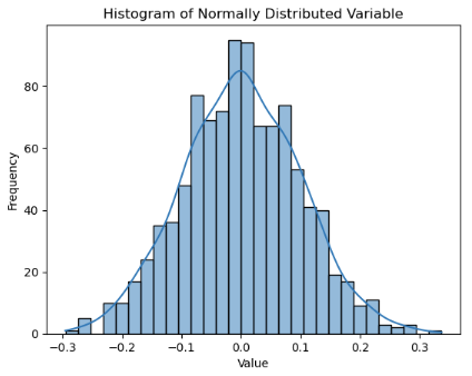
Observe that the var feature is normally distributed, where the mean and the median (50% percentile) are expected to be more or less equal. For skewed distributions, the mean tends to lean towards the heavier tail.
However, these are heuristic checks and actual determination are done using specific statistical tests like Shapiro-Wilk test or Kolmogorov-Smirnov test for normality.
Binomial distribution
Suppose you want to understand how well a particular characteristic is being observed in a group of penguins.
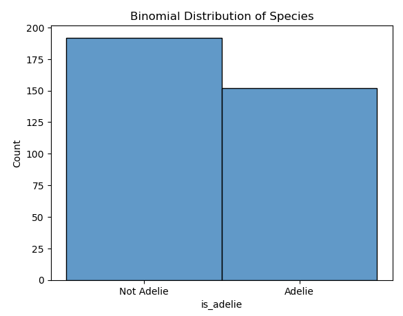
You decide to examine a dataset of 200 penguins to see if they are of the Adelie species. This is a binomial distribution problem because there are two possible outcomes (Adelie or not Adelie), a fixed number of trials (200 penguins), and each trial is independent of others.
After analyzing the dataset, you find that 150 penguins are of the Adelie species.
Knowing that your data follows a binomial distribution allows you to make predictions about future datasets or groups of penguins. For example, if you study another group of 200 penguins, you can expect around 150 to be of the Adelie species.
The following Python code plots a histogram of the is_adelie binomial variable. The discrete=True argument in sns.histplot ensures that the bins are treated as discrete intervals. This means that each bar in the histogram corresponds exactly to one category or boolean value, making the plot easier to interpret.
import seaborn as sns
import matplotlib.pyplot as plt
import numpy as np

# Load the Penguins dataset from seaborn
penguins = sns.load_dataset('penguins')

# Create a binomial variable for 'species'
penguins['is_adelie'] = np.where(penguins['species'] == 'Adelie', 1, 0)

# Plot the distribution of 'is_adelie'
sns.histplot(data=penguins, x='is_adelie', bins=2, discrete=True)
plt.title('Binomial Distribution of Species')
plt.xticks([0, 1], ['Not Adelie', 'Adelie'])
plt.show()
Uniform distribution
A uniform distribution, also known as a rectangular distribution, is a type of probability distribution in which all outcomes are equally likely. Each interval of the same length on the distribution’s support has the same probability.
import numpy as np
import matplotlib.pyplot as plt

# Generate a uniform distribution
uniform_data = np.random.uniform(-1, 1, 1000)

# Plot the distribution
plt.hist(uniform_data, bins=20, density=True)
plt.title('Uniform Distribution')
plt.xlabel('Value')
plt.ylabel('Frequency')
plt.show()
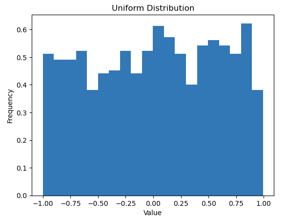
In this code, the np.random.uniform function generates 1000 random numbers that are uniformly distributed between -1 and 1. The bins=30 argument specifies that the data should be divided into 30 bins, and density=True ensures that the histogram is normalized to form a probability density. This means the area under the histogram integrates to 1, which is useful when comparing distributions.
Note
You'll likely get different results if you run the code multiple times. The basic idea of randomness is that it's unpredictable, and each time you sample, you can get different results.
You can control this process by setting a seed value with np.random.seed. This is very useful for testing and debugging in the model building phase, as it allows you to reproduce the same results.