Previous

Next

Exercise: Integrate SQL and spark pools in Azure Synapse Analytics

Completed

In the following exercise, we will explore integrating SQL and Apache Spark pools in Azure Synapse Analytics.

Integrating SQL and Apache Spark pools in Azure Synapse Analytics

You want to write to a dedicated SQL pool after performing data engineering tasks in Spark, then reference the SQL pool data as a source for joining with Apache Spark DataFrames that contain data from other files.

You decide to use the Azure Synapse Apache Spark to Synapse SQL connector to efficiently transfer data between Spark pools and SQL pools in Azure Synapse.

Transferring data between Apache Spark pools and SQL pools can be done using JavaDataBaseConnectivity (JDBC). However, given two distributed systems such as Apache Spark and SQL pools, JDBC tends to be a bottleneck with serial data transfer.

The Azure Synapse Apache Spark pool to Synapse SQL connector is a data source implementation for Apache Spark. It uses the Azure Data Lake Storage Gen2 and PolyBase in SQL pools to efficiently transfer data between the Spark cluster and the Synapse SQL instance.

1. If we want to use the Apache Spark pool to Synapse SQL connector (sqlanalytics), one option is to create a temporary view of the data within the DataFrame. Execute the code below in a new cell to create a view named top_purchases:

   # Create a temporary view for top purchases 
   topPurchases.createOrReplaceTempView("top_purchases")
   

   We created a new temporary view from the topPurchases dataframe that we created earlier and which contains the flattened JSON user purchases data.

2. We must execute code that uses the Apache Spark pool to Synapse SQL connector in Scala. To do so, we add the %%spark magic to the cell. Execute the code below in a new cell to read from the top_purchases view:

   %%spark
   // Make sure the name of the SQL pool (SQLPool01 below) matches the name of your SQL pool.
   val df = spark.sqlContext.sql("select * from top_purchases")
   df.write.sqlanalytics("SQLPool01.wwi.TopPurchases", Constants.INTERNAL)
   

   Note

   The cell may take over a minute to execute. If you have run this command before, you will receive an error stating that "There is already and object named..." because the table already exists.

   After the cell finishes executing, let's take a look at the list of SQL pool tables to verify that the table was successfully created for us.

3. Leave the notebook open, then navigate to the Data hub (if not already selected).

   

4. Select the Workspace tab (1), expand the SQL pool, select the ellipses (...) on Tables (2) and select Refresh (3). Expand the wwi.TopPurchases table and columns (4).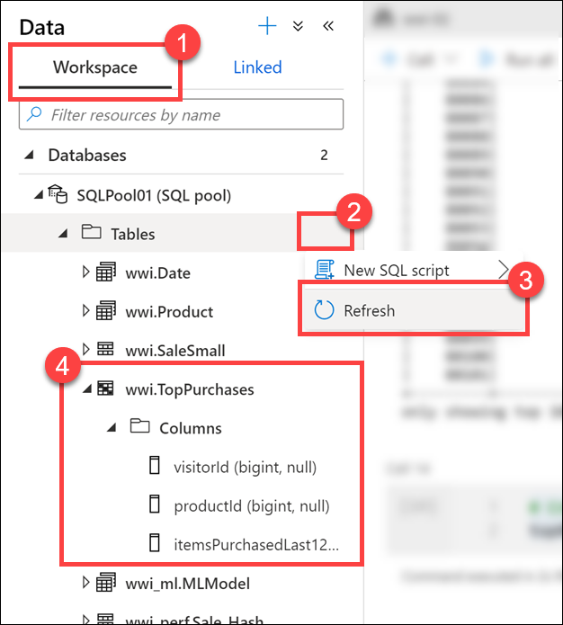

   

   As you can see, the wwi.TopPurchases table was automatically created for us, based on the derived schema of the Apache Spark DataFrame. The Apache Spark pool to Synapse SQL connector was responsible for creating the table and efficiently loading the data into it.

5. Return to the notebook and execute the code below in a new cell to read sales data from all the Parquet files located in the sale-small/Year=2019/Quarter=Q4/Month=12/ folder:

   dfsales = spark.read.load('abfss://wwi-02@' + datalake + '.dfs.core.windows.net/sale-small/Year=2019/Quarter=Q4/Month=12/*/*.parquet', format='parquet')
   display(dfsales.limit(10))
   

   Note

   It can take over 3 minutes for this cell to execute.

   The datalake variable we created in the first cell is used here as part of the file path.

   

   Compare the file path in the cell above to the file path in the first cell. Here we are using a relative path to load all December 2019 sales data from the Parquet files located in sale-small, vs. just December 31, 2010 sales data.

   Next, let's load the TopSales data from the SQL pool table we created earlier into a new Apache Spark DataFrame, then join it with this new dfsales DataFrame. To do so, we must once again use the %%spark magic on a new cell since we'll use the Apache Spark pool to Synapse SQL connector to retrieve data from the SQL pool. Then we need to add the DataFrame contents to a new temporary view so we can access the data from Python.

6. Execute the code below in a new cell to read from the TopSales SQL pool table and save it to a temporary view:

   %%spark
   // Make sure the name of the SQL pool (SQLPool01 below) matches the name of your SQL pool.
   val df2 = spark.read.sqlanalytics("SQLPool01.wwi.TopPurchases")
   df2.createTempView("top_purchases_sql")
   
   df2.head(10)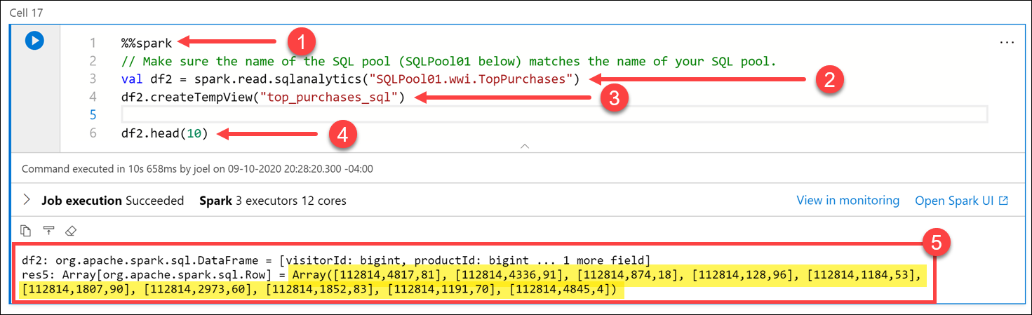
   

   

   The cell's language is set to Scala by using the %%spark magic (1) at the top of the cell. We declared a new variable named df2 as a new DataFrame created by the spark.read.sqlanalytics method, which reads from the TopPurchases table (2) in the SQL pool. Then we populated a new temporary view named top_purchases_sql (3). Finally, we showed the first 10 records with the df2.head(10)) line (4). The cell output displays the DataFrame values (5).

7. Execute the code below in a new cell to create a new DataFrame in Python from the top_purchases_sql temporary view, then display the first 10 results:

   dfTopPurchasesFromSql = sqlContext.table("top_purchases_sql")
   
   display(dfTopPurchasesFromSql.limit(10))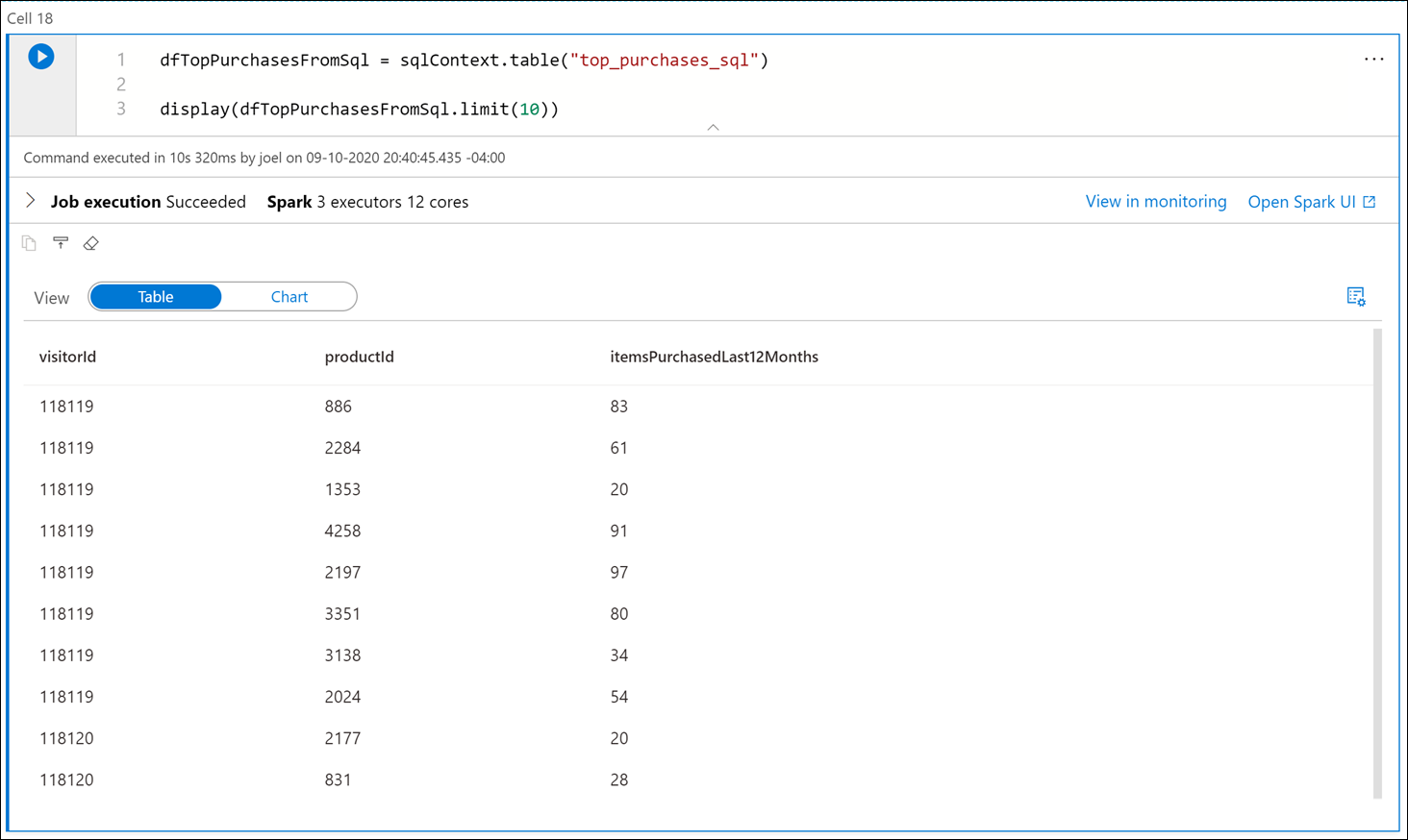
   

   

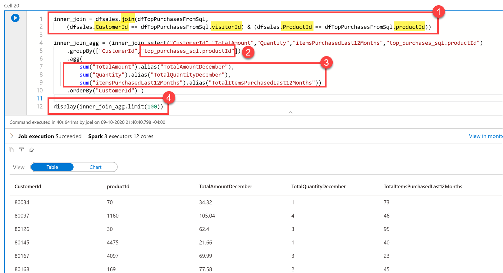
8. Execute the code below in a new cell to join the data from the sales Parquet files and the TopPurchases SQL pool:

   inner_join = dfsales.join(dfTopPurchasesFromSql,
       (dfsales.CustomerId == dfTopPurchasesFromSql.visitorId) & (dfsales.ProductId == dfTopPurchasesFromSql.productId))
   
   inner_join_agg = (inner_join.select("CustomerId","TotalAmount","Quantity","itemsPurchasedLast12Months","top_purchases_sql.productId")
       .groupBy(["CustomerId","top_purchases_sql.productId"])
       .agg(
           sum("TotalAmount").alias("TotalAmountDecember"),
           sum("Quantity").alias("TotalQuantityDecember"),
           sum("itemsPurchasedLast12Months").alias("TotalItemsPurchasedLast12Months"))
       .orderBy("CustomerId") )
   
   display(inner_join_agg.limit(100))
   

   In the query, we joined the dfsales and dfTopPurchasesFromSql DataFrames, matching on CustomerId and ProductId. This join combined the TopPurchases SQL pool table data with the December 2019 sales Parquet data (1).

   We grouped by the CustomerId and ProductId fields. Since the ProductId field name is ambiguous (it exists in both DataFrames), we had to fully qualify the ProductId name to refer to the one in the TopPurchases DataFrame (2).

   Then we created an aggregate that summed the total amount spent on each product in December, the total number of product items in December, and the total product items purchased in the last 12 months (3).

   Finally, we displayed the joined and aggregated data in a table view.

   Feel free to select the column headers in the Table view to sort the result set.

   

Continue