Optimize models by using gradient descent
We've seen how cost functions evaluate how well models perform by using data. The optimizer is the final piece of the puzzle.
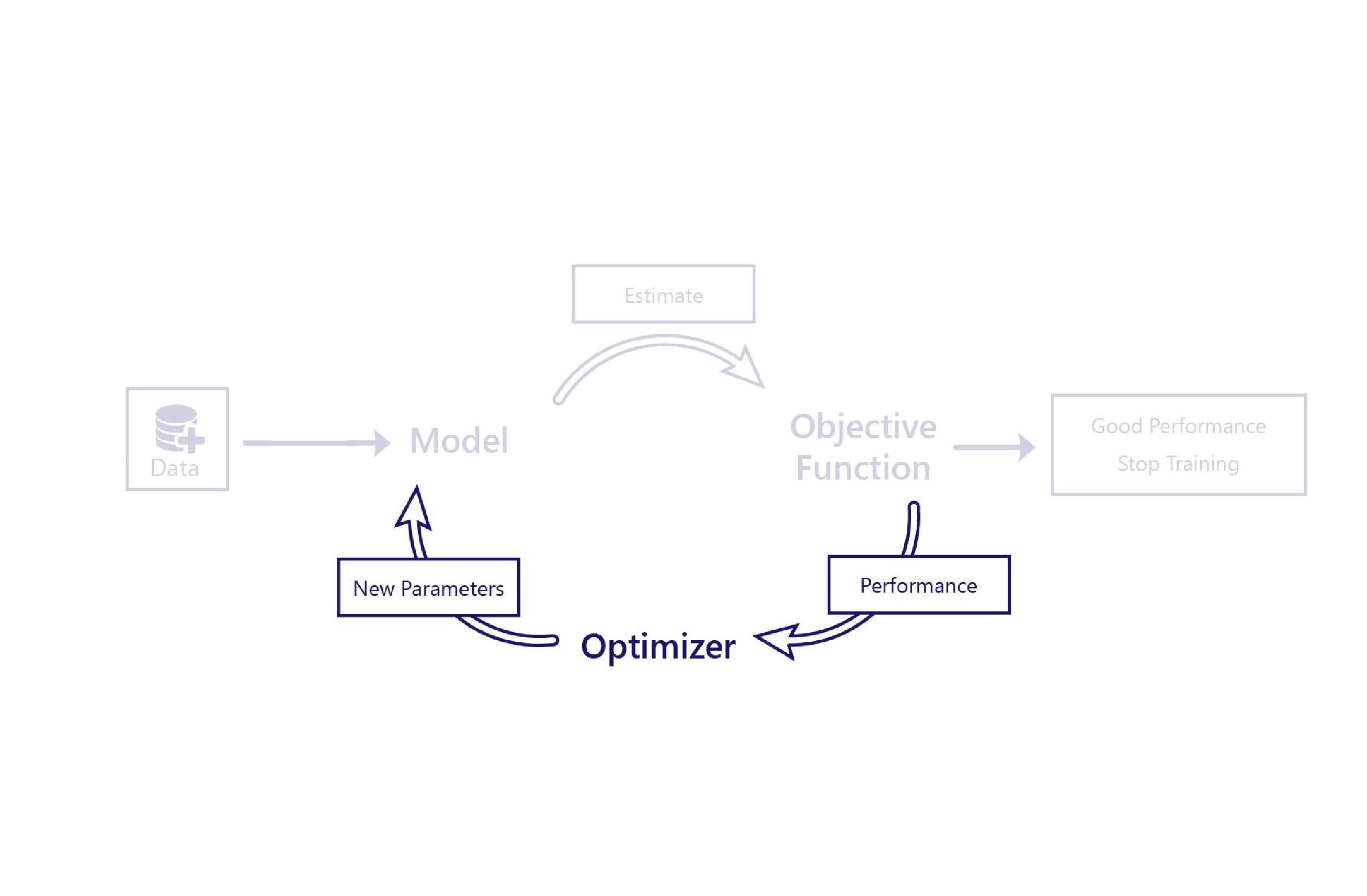
The optimizer's role is to alter the model in a way that improves its performance. It does this alteration by inspecting the model outputs and cost and suggesting new parameters for the model.
For example, in our farming scenario, our linear model has two parameters: the line's intercept and the line's slope. If the line's intercept is wrong, the model underestimates or overestimates temperatures on average. If the slope is set wrong, the model won't do a good job of demonstrating how temperatures have changed since the 1950s. The optimizer changes these two parameters so that they do an optimal job of modeling temperatures over time.
Gradient descent
The most common optimization algorithm today is gradient descent. Several variants of this algorithm exist, but they all use the same core concepts.
Gradient descent uses calculus to estimate how changing each parameter changes the cost. For example, increasing a parameter might be predicted to reduce the cost.
Gradient descent is named as such because it calculates the gradient (slope) of the relationship between each model parameter and the cost. The parameters are then altered to move down this slope.
This algorithm is simple and powerful, yet it isn't guaranteed to find the optimal model parameters that minimize the cost. The two main sources of error are local minima and instability.
Local minima
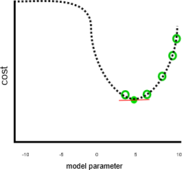
Our previous example looked to do a good job, assuming that cost would have kept increasing when the parameter was smaller than 0 or greater than 10:
This job wouldn't have been so great if parameters smaller than zero or larger than 10 would have resulted in lower costs, like in this image:
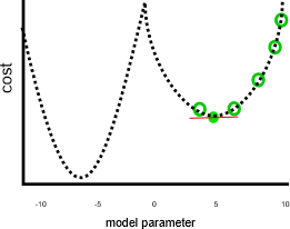
In the preceding graph, a parameter value of negative seven would have been a better solution than five, because it has a lower cost. Gradient descent doesn't know the full relationship between each parameter and the cost—which is represented by the dotted line—in advance. Therefore, it's prone to finding local minima: parameter estimates that aren't the best solution, but the gradient is zero.
Instability
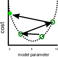
A related issue is that gradient descent sometimes shows instability. This instability usually occurs when the step size or learning rate—the amount that each parameter is adjusted by each iteration—is too large. The parameters are then adjusted too far on each step, and the model actually gets worse with each iteration:
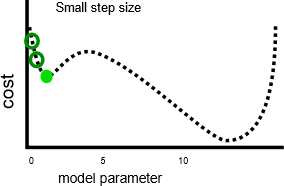
Having a slower learning rate can solve this problem, but might also introduce issues. First, slower learning rates can mean training takes a long time, because more steps are required. Second, taking smaller steps makes it more likely that training settles on a local minima:
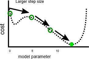
By contrast, a faster learning rate can make it easier to avoid hitting local minima, because larger steps can skip over local maxima:
As we'll see in the next exercise, there's an optimal step size for each problem. Finding this optimum is something that often requires experimentation.