Explore data load strategies
In Microsoft Fabric, there are many ways you can choose to load data in a warehouse. This step is fundamental as it ensures that high-quality, transformed or processed data is integrated into a single repository.
Also, the efficiency of data loading directly impacts the timeliness and accuracy of analytics, making it vital for real-time decision-making processes. Investing time and resources in designing and implementing a robust data loading strategy is essential for the success of the data warehouse project.
Understand data ingestion and data load operations
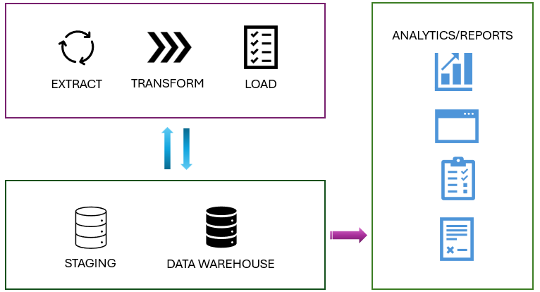
While both processes are part of the ETL (Extract, Transform, Load) pipeline in a data warehouse scenario, they usually serve different purposes. Data ingestion/extract is about moving raw data from various sources into a central repository. On the other hand, data loading involves taking the transformed or processed data and loading it into the final storage destination for analysis and reporting.
All Fabric data items like data warehouses and lakehouses store their data automatically in OneLake in Delta Parquet format.
Stage your data
You may have to build and work with auxiliary objects involved in a load operation such as tables, stored procedures, and functions. These auxiliary objects are commonly referred to as staging. Staging objects act as temporary storage and transformation areas. They can share resources with a data warehouse, or live in its own storage area.
Staging serves as an abstraction layer, simplifying and facilitating the load operation to the final tables in the data warehouse.
Also, staging area provides a buffer that can help to minimize the impact of the load operation on the performance of the data warehouse. This is important in environments where the data warehouse needs to remain operational and responsive during the data loading process.
Review type of data loads
There are two types of data loads to consider when loading a data warehouse.
| Load Type | Description | Operation | Duration | Complexity | Best used |
|---|---|---|---|---|---|
| Full (initial) load | The process of populating the data warehouse for the first time. | All the tables are truncated and reloaded, and the old data is lost | It may take longer to complete due to the amount of data being handled | Easier to implement as there's no history preserved | This method is typically used when setting up a new data warehouse, or when a complete refresh of the data is required |
| Incremental load | The process of updating the data warehouse with the changes since the last update | The history is preserved, and tables are updated with new information | Takes less time than the initial load | Implementation is more complex than the initial load | This method is commonly used for regular updates to the data warehouse, such as daily or hourly updates. It requires mechanisms to track changes in the source data since the last load. |
An ETL (Extract, Transform, Load) process for a data warehouse doesn't always need both the full load and the incremental load. In some cases, a combination of both methods might be used. The choice between a full load and an incremental load depends on many factors such as the amount of data, the characteristics of the data, and the requirements of the data warehouse.
To learn more about how to perform an incremental load, see Incremental load.
Load a dimension table
Think of a dimension table as the "who, what, where, when, why” of your data warehouse. It’s like the descriptive backdrop that gives context to the raw numbers found in the fact tables.
For example, if you’re running an online store, your fact table might contain the raw sales data - how many units of each product were sold. But without a dimension table, you wouldn’t know who bought those products, when they were bought, or where the buyer is located.
Slowly changing dimensions (SCD)
Slowly Changing Dimensions change over time, but at a slow pace and unpredictably. For example, a customer’s address in a retail business. When a customer moves, their address changes. If you overwrite the old address with the new one, you lose the history. But if you want to analyze historical sales data, you might need to know where the customer lived at the time of each sale. This is where SCDs come into play.
There are several types of slowly changing dimensions in a data warehouse, with type 1 and type 2 being the most frequently used.
- Type 0 SCD: The dimension attributes never change.
- Type 1 SCD: Overwrites existing data, doesn't keep history.
- Type 2 SCD: Adds new records for changes, keeps full history for a given natural key.
- Type 3 SCD: History is added as a new column.
- Type 4 SCD: A new dimension is added.
- Type 5 SCD: When certain attributes of a large dimension change over time, but using type 2 isn't feasible due to the dimension’s large size.
- Type 6 SCD: Combination of type 2 and type 3.
In type 2 SCD, when a new version of the same element is brought to the data warehouse, the old version is considered expired and the new one becomes active.

The following example shows how to handle changes in a type 2 SCD for the Dim_Products table using T-SQL.
IF EXISTS (SELECT 1 FROM Dim_Products WHERE SourceKey = @ProductID AND IsActive = 'True')
BEGIN
    -- Existing product record
    UPDATE Dim_Products
    SET ValidTo = GETDATE(), IsActive = 'False'
    WHERE SourceKey = @ProductID AND IsActive = 'True';
END
ELSE
BEGIN
    -- New product record
    INSERT INTO Dim_Products (SourceKey, ProductName, StartDate, EndDate, IsActive)
    VALUES (@ProductID, @ProductName, GETDATE(), '9999-12-31', 'True');
END
The mechanism for detecting changes in source systems is crucial for determining when records are inserted, updated, or deleted. Change Data Capture (CDC), change tracking, and triggers are all features available for managing data tracking in source systems such as SQL Server.
Load a fact table
Let's consider an example where we load a Fact_Sales table in a data warehouse. This table contains sales transactions data with columns such as FactKey, DateKey, ProductKey, OrderID, Quantity, Price, and LoadTime.
Assume we have a source table Order_Detail in an OLTP system with columns: OrderID, OrderDate, ProductID, Quantity, and Price.
The following T-SQL script example load the Fact_Sales table.
-- Lookup keys in dimension tables
INSERT INTO Fact_Sales (DateKey, ProductKey, OrderID, Quantity, Price, LoadTime)
SELECT d.DateKey, p.ProductKey, o.OrderID, o.Quantity, o.Price, GETDATE()
FROM Order_Detail o
JOIN Dim_Date d ON o.OrderDate = d.Date
JOIN Dim_Product p ON o.ProductID = p.ProductID;
In this example, we use a JOIN operation to look up the DateKey and ProductKey values in the Dim_Date and Dim_Product tables, respectively, and then insert the data into the Fact_Sales table. However, it is important to note that the complexity of the loading process depends on several factors, including the amount of data, the transformation requirements, error handling, schema differences, and performance.