Understand PCA and import the dataset
Principal component analysis (PCA) is an algorithm that helps us get a dataset into working condition by removing dimensions that must be calculated in an analysis of the dataset.
PCA in theory
One way we reduce the number of dimensions we have to work with is by reducing the number of features considered in an analysis. PCA provides another way: reducing the number of dimensions that we have to work with by projecting our feature space into a lower-dimensional space. We can do this because in most real-world problems, data points aren't spread uniformly across all dimensions. Although some features might be nearly constant, others are highly correlated. The highly correlated data points lie close to a lower-dimensional subspace.
In the following image, the data points aren't spread across the entire plane, but are clumped roughly in an oval. Because the cluster (or any cluster) is roughly elliptical, it can be mathematically described by two values: its major (long) axis and its minor (short) axis. These axes form the principal components of the cluster.
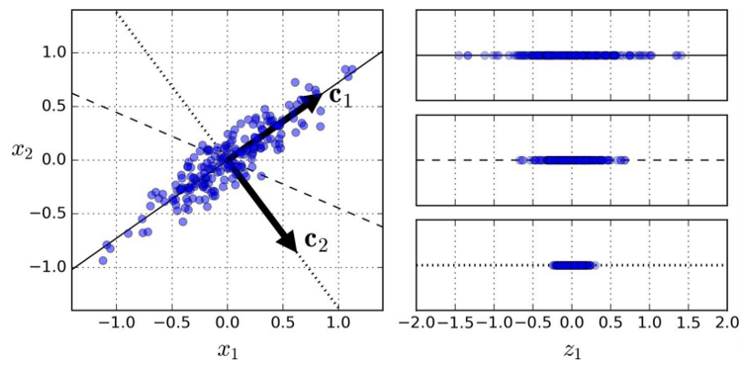
We can construct a whole new feature space around this cluster that's defined by two eigenvectors: $c_{1}$ and $c_{2}$. Eigenvectors are the vectors that define the linear transformation to this new feature space.
Better still, we don't have to consider all of the dimensions of this new space. Intuitively, we can see that most of the points lie on or close to the line that runs through $c_{1}$. If we project the cluster down from two dimensions to that single dimension, we capture most of the information about this dataset while simplifying our analysis. This ability to extract most of the information from a dataset by considering only a fraction of its definitive eigenvectors forms the heart of PCA.
Import modules and dataset
You must first clean and prepare the data to conduct PCA on it, so pandas will be essential. You also need NumPy, a bit of scikit-learn, and pyplot.
To add these libraries, run this code:
import pandas as pd
import numpy as np
from sklearn.decomposition import PCA
from sklearn.preprocessing import StandardScaler
import matplotlib.pyplot as plt
%matplotlib inline
The dataset we'll use here's the same one that's drawn from the U.S. Department of Agriculture National Nutrient Database for Standard Reference that you prepared in the preceding module.
Remember to set the encoding to latin1 (for µg):
df = pd.read_csv('Data/USDA-nndb-combined.csv', encoding='latin1')
We can check the number of columns and rows by using the info() method for the DataFrame:
df.info()
The output is:
<class 'pandas.core.frame.DataFrame'>
RangeIndex: 8989 entries, 0 to 8988
Data columns (total 54 columns):
 #   Column             Non-Null Count  Dtype
---  ------             --------------  -----
 0   NDB_No             8989 non-null   int64
 1   FoodGroup          8618 non-null   object
 2   Shrt_Desc          8790 non-null   object
 3   Water_(g)          8789 non-null   float64
 4   Energ_Kcal         8790 non-null   float64
 5   Protein_(g)        8790 non-null   float64
 6   Lipid_Tot_(g)      8790 non-null   float64
 7   Ash_(g)            8465 non-null   float64
 8   Carbohydrt_(g)     8790 non-null   float64
 9   Fiber_TD_(g)       8196 non-null   float64
 10  Sugar_Tot_(g)      6958 non-null   float64
 11  Calcium_(mg)       8442 non-null   float64
 12  Iron_(mg)          8646 non-null   float64
 13  Magnesium_(mg)     8051 non-null   float64
 14  Phosphorus_(mg)    8211 non-null   float64
 15  Potassium_(mg)     8364 non-null   float64
 16  Sodium_(mg)        8707 non-null   float64
 17  Zinc_(mg)          8084 non-null   float64
 18  Copper_mg)         7533 non-null   float64
 19  Manganese_(mg)     6630 non-null   float64
 20  Selenium_(µg)     7090 non-null   float64
 21  Vit_C_(mg)         7972 non-null   float64
 22  Thiamin_(mg)       8156 non-null   float64
 23  Riboflavin_(mg)    8174 non-null   float64
 24  Niacin_(mg)        8153 non-null   float64
 25  Panto_Acid_mg)     6548 non-null   float64
 26  Vit_B6_(mg)        7885 non-null   float64
 27  Folate_Tot_(µg)   7529 non-null   float64
 28  Folic_Acid_(µg)   6751 non-null   float64
 29  Food_Folate_(µg)  7022 non-null   float64
 30  Folate_DFE_(µg)   6733 non-null   float64
 31  Choline_Tot_ (mg)  4774 non-null   float64
 32  Vit_B12_(µg)      7597 non-null   float64
 33  Vit_A_IU           8079 non-null   float64
 34  Vit_A_RAE          7255 non-null   float64
 35  Retinol_(µg)      6984 non-null   float64
 36  Alpha_Carot_(µg)  5532 non-null   float64
 37  Beta_Carot_(µg)   5628 non-null   float64
 38  Beta_Crypt_(µg)   5520 non-null   float64
 39  Lycopene_(µg)     5498 non-null   float64
 40  Lut+Zea_ (µg)     5475 non-null   float64
 41  Vit_E_(mg)         5901 non-null   float64
 42  Vit_D_µg          5528 non-null   float64
 43  Vit_D_IU           5579 non-null   float64
 44  Vit_K_(µg)        5227 non-null   float64
 45  FA_Sat_(g)         8441 non-null   float64
 46  FA_Mono_(g)        8124 non-null   float64
 47  FA_Poly_(g)        8125 non-null   float64
 48  Cholestrl_(mg)     8380 non-null   float64
 49  GmWt_1             8490 non-null   float64
 50  GmWt_Desc1         8491 non-null   object
 51  GmWt_2             4825 non-null   float64
 52  GmWt_Desc2         4825 non-null   object
 53  Refuse_Pct         8740 non-null   float64
dtypes: float64(49), int64(1), object(4)
memory usage: 3.7+ MB
Try it yourself
Can you think of a more concise way to check the number of rows and columns in a DataFrame?
Use one of the attributes of the DataFrame.
Here's a possible solution:
df.count(axis='columns')
The output is:
0       54
1       54
2       54
3       54
4       54
        ..
8984    49
8985    50
8986    53
8987    48
8988    49
Length: 8989, dtype: int64