Use Tidyverse
Tidyverse is a collection of R packages that data scientists commonly use in everyday data analyses. It includes packages for data import (readr), data visualization (ggplot2), data manipulation (dplyr, tidyr), functional programming (purrr), and model building (tidymodels) etc. The packages in tidyverse are designed to work together seamlessly and follow a consistent set of design principles.
Microsoft Fabric distributes the latest stable version of tidyverse with every runtime release. Import and start using your familiar R packages.
Prerequisites
Get a Microsoft Fabric subscription. Or, sign up for a free Microsoft Fabric trial.
Sign in to Microsoft Fabric.
Use the experience switcher on the left side of your home page to switch to the Synapse Data Science experience.
Open or create a notebook. To learn how, see How to use Microsoft Fabric notebooks.
Set the language option to SparkR (R) to change the primary language.
Attach your notebook to a lakehouse. On the left side, select Add to add an existing lakehouse or to create a lakehouse.
Load tidyverse
# load tidyverse
library(tidyverse)
Data import
readr is an R package that provides tools for reading rectangular data files such as CSV, TSV, and fixed-width files. readr provides a fast and friendly way to read rectangular data files such as providing functions read_csv() and read_tsv() for reading CSV and TSV files respectively.
Let's first create an R data.frame, write it to lakehouse using readr::write_csv() and read it back with readr::read_csv().
Note
To access Lakehouse files using readr, you need to use the File API path. In the Lakehouse explorer, right click on the file or folder that you want to access and copy its File API path from the contextual menu.
# create an R data frame
set.seed(1)
stocks <- data.frame(
   time = as.Date('2009-01-01') + 0:9,
   X = rnorm(10, 20, 1),
   Y = rnorm(10, 20, 2),
   Z = rnorm(10, 20, 4)
 )
stocks
Then let's write the data to lakehouse using the File API path.
# write data to lakehouse using the File API path
temp_csv_api <- "/lakehouse/default/Files/stocks.csv"
readr::write_csv(stocks,temp_csv_api)
Read the data from lakehouse.
# read data from lakehouse using the File API path
stocks_readr <- readr::read_csv(temp_csv_api)

# show the content of the R date.frame
head(stocks_readr)
Data tidying
tidyr is an R package that provides tools for working with messy data. The main functions in tidyr are designed to help you reshape data into a tidy format. Tidy data has a specific structure where each variable is a column and each observation is a row, which makes it easier to work with data in R and other tools.
For example, the gather() function in tidyr can be used to convert wide data into long data. Here's an example:
# convert the stock data into longer data
library(tidyr)
stocksL <- gather(data = stocks, key = stock, value = price, X, Y, Z)
stocksL
Functional programming
purrr is an R package that enhances R’s functional programming toolkit by providing a complete and consistent set of tools for working with functions and vectors. The best place to start with purrr is the family of map() functions that allow you to replace many for loops with code that is both more succinct and easier to read. Here’s an example of using map() to apply a function to each element of a list:
# double the stock values using purrr
library(purrr)
stocks_double = map(stocks %>% select_if(is.numeric), ~.x*2)
stocks_double
Data manipulation
dplyr is an R package that provides a consistent set of verbs that help you solve the most common data manipulation problems, such as selecting variables based on the names, picking cases based on the values, reducing multiple values down to a single summary, and changing the ordering of the rows etc. Here are some examples:
#  pick variables based on their names using select()
stocks_value <- stocks %>% select(X:Z)
stocks_value
# pick cases based on their values using filter()
filter(stocks_value, X >20)
# add new variables that are functions of existing variables using mutate()
library(lubridate)

stocks_wday <- stocks %>%
    select(time:Z) %>%
    mutate(
        weekday = wday(time)
    )

stocks_wday
# change the ordering of the rows using arrange()
arrange(stocks_wday, weekday)
# reduce multiple values down to a single summary using summarise()
stocks_wday %>%
    group_by(weekday) %>%
    summarize(meanX = mean(X), n= n())
Data visualization
ggplot2 is an R package for declaratively creating graphics, based on The Grammar of Graphics. You provide the data, tell ggplot2 how to map variables to aesthetics, what graphical primitives to use, and it takes care of the details. Here are some examples:
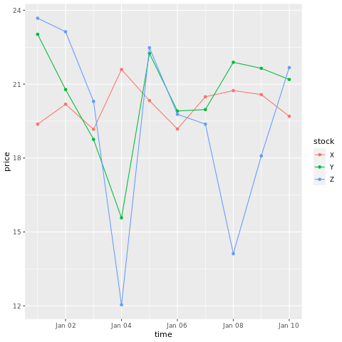
# draw a chart with points and lines all in one

ggplot(stocksL, aes(x=time, y=price, colour = stock)) +
  geom_point()+
  geom_line()
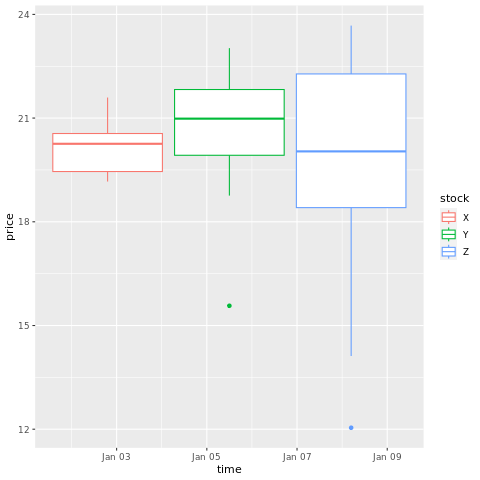
# draw a boxplot

ggplot(stocksL, aes(x=time, y=price, colour = stock)) +
  geom_boxplot()
Model building
The tidymodels framework is a collection of packages for modeling and machine learning using tidyverse principles. It covers a list of core packages for a wide variety of model building tasks, such as rsample for train/test dataset sample splitting, parsnip for model specification, recipes for data preprocessing, workflows for modeling workflows, tune for hyperparameters tuning, yardstick for model evaluation, broom for tiding model outputs, and dials for managing tuning parameters. You can learn more about the packages by visiting tidymodels website. Here's an example of building a linear regression model to predict the miles per gallon (mpg) of a car based on its weight (wt):
# look at the relationship between the miles per gallon (mpg) of a car and its weight (wt)
ggplot(mtcars, aes(wt,mpg))+
geom_point()
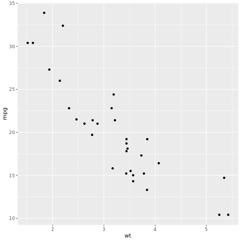
From the scatterplot, the relationship looks approximately linear and the variance looks constant. Let's try to model this using linear regression.
library(tidymodels)

# split test and training dataset
set.seed(123)
split <- initial_split(mtcars, prop = 0.7, strata = "cyl")
train <- training(split)
test <- testing(split)


# config the linear regression model
lm_spec <- linear_reg() %>%
  set_engine("lm") %>%
  set_mode("regression")

# build the model
lm_fit <- lm_spec %>%
  fit(mpg ~ wt, data = train)

tidy(lm_fit)
Apply the linear regression model to predict on test dataset.
# using the lm model to predict on test dataset
predictions <- predict(lm_fit, test)
predictions
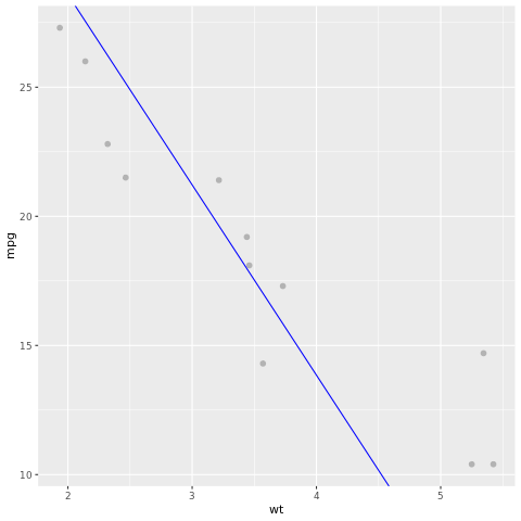
Let's take a look at the model result. We can draw the model as a line chart and the test ground truth data as points on the same chart. The model looks good.
# draw the model as a line chart and the test data groundtruth as points
lm_aug <- augment(lm_fit, test)
ggplot(lm_aug, aes(x = wt, y = mpg)) +
  geom_point(size=2,color="grey70") +
  geom_abline(intercept = lm_fit$fit$coefficients[1], slope = lm_fit$fit$coefficients[2], color = "blue")
Related content
Feedback
Coming soon: Throughout 2024 we will be phasing out GitHub Issues as the feedback mechanism for content and replacing it with a new feedback system. For more information see: https://aka.ms/ContentUserFeedback.
Submit and view feedback for