How To: Show pivot table data in flat format
As a seasoned Excel user, you are no doubt familiar with Pivot Tables and how they work. (If not, here's a great place to get started on them: https://office.microsoft.com/en-us/excel-help/pivottable-reports-101-HA001034632.aspx). Perhaps you've wanted to see your pivot table data differently. We know how to pivot the tables to display our data as needed, but what if we need to see all of the data for a field in a single flat format? How can we do this?
Consider the following sample pivot table:
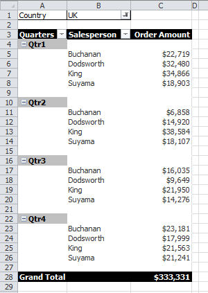
In order to show the data in flat file format, we need to be showing Grand Totals as we are with this table. If you aren't seeing grand totals, right click in your pivot table, left click PivotTable options. Click the 'Totals & Filters' tab and make sure both 'Show grand totals for rows' and 'Show grand totals for columns' are checked.
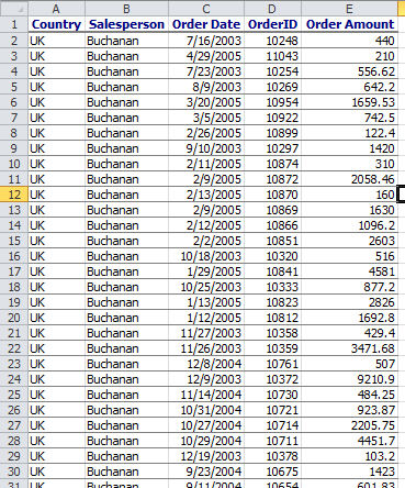
To display the data in a flat format, just double click the Grand total. What you get is the flat data (like the sample below) on a new tab added to your workbook.
Comments
Anonymous
September 25, 2012
This doesn't give you a flat file though - it just gives you the data you stuck into the table in the original format. if you want to do sum/count/any aggregation (the reason you create a pivot in the first place) then this doesn't seem to work.Anonymous
October 16, 2012
I agree with Sam, this didn't solve my problem at all.Anonymous
July 24, 2013
It did solve my problem to see all data behind a pivot table I did not createAnonymous
November 08, 2013
Figured this out It's under PivotTable Tools > Design > Report Layout > Show in Tabular Form- Anonymous
June 30, 2016
Wow, I love the results. Got what I wanted.
- Anonymous
Anonymous
May 19, 2014
PivotGrid control for Windows Forms, http://www.kettic.com/winforms_ui/pivotgrid.shtmlAnonymous
March 22, 2016
Exactly what I was looking for.Thank you!- Anonymous
March 08, 2017
- In the source, use the CONCATENATE function to put all the fields in a single field with delimiters. E.g., =CONCATENATE(I2,",",N2,",",G2,",",A2)- Do your Aggregating in the Pivot table against that single concat field- Copy Pivot Table to a new excel- Save as CSV- Open in a text editor and remove the "" around the Concate field and add the headers. If you have actual commas in yuor content use a different delimiter and then find/replace it accounting for the quotes.
- Anonymous
Anonymous
August 18, 2016
This is genius - thank you! So simple. 2 clicks.Anonymous
September 21, 2016
This works great when using pivot tables as a poor man's query.